Parallel computing with Python

Questions

• What is parallel computing?

• What are the different parallelization mechanisms for Python?

• How to implement parallel algorithms in Python code?

• How to deploy threads and workers at our HPC centers?

Objectives

• Learn general concepts for parallel computing

• Gain knowledge on the tools for parallel programming in different languages

• Familiarize with the tools to monitor the usage of resources

Get today’s tarball!

Use the tarball with exercises

Prerequisites

• Demo

HPC2NUPPMAXNSCLUNARCPDC

• If not already done so:

$ ml GCCcore/11.2.0 Python/3.9.6

$ python -m venv vpyenv-python-course

$ source /proj/nobackup/<your-project-storage>/vpyenv-python-course/bin/activate

• For the numba example install the corresponding module:

$ pip install numba

• For the mpi4py example add the following modules:

$ ml GCC/11.2.0 OpenMPI/4.1.1

$ pip install mpi4py

• For the Julia example we will need PyJulia:

$ ml Julia/1.9.3-linux-x86_64

$ pip install julia

• Start Python on the command line and type:

>>> import julia
>>> julia.install()

This will install the PyCall connector between Python and Julia.

• For the Heat examples:

$ ml GCC/11.2.0 OpenMPI/4.1.1
$ ml CUDA/12.0.0
$ pip install torch --index-url https://download.pytorch.org/whl/cu126
$ pip install heat[hdf5,netcdf]

• The PyOMP example needs an additional package:

$ pip install pyomp

• Quit Python, you should be ready to go!

What is parallel programming?

Parallel programming is the science and art of writing code that execute tasks on different computing units (cores) simultaneously. In the past computers were shiped with a single core per Central Processing Unit (CPU) and therefore only a single computation at the time (serial program) could be executed.

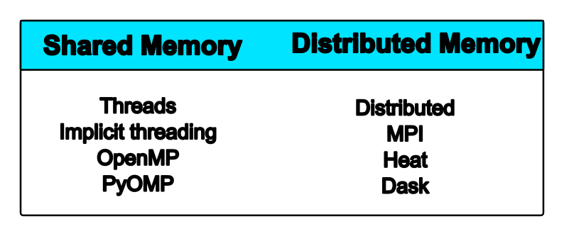
Nowadays computer architectures are more complex than the single core CPU mentioned already. For instance, common architectures include those where several cores in a CPU share a common memory space and also those where CPUs are connected through some network interconnect.

Shared Memory and Distributed Memory architectures.

A more realistic picture of a computer architecture can be seen in the following picture where we have 14 cores that shared a common memory of 64 GB. These cores form the socket and the two sockets shown in this picture constitute a node.

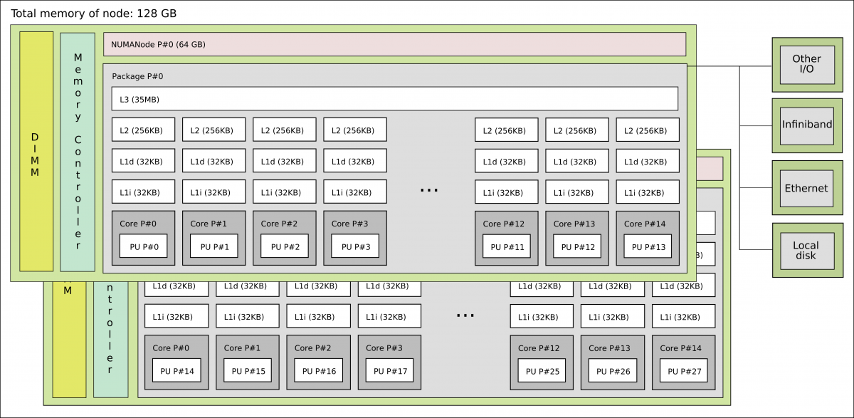
1 standard node on Kebnekaise @HPC2N

It is interesting to notice that there are different types of memory available for the cores, ranging from the L1 cache to the node’s memory for a single node. In the former, the bandwidth can be TB/s while in the latter GB/s.

Now you can see that on a single node you already have several computing units (cores) and also a hierarchy of memory resources which is denoted as Non Uniform Memory Access (NUMA).

Besides the standard CPUs, nowadays one finds Graphic Processing Units (GPUs) architectures in HPC clusters.

Why is parallel programming needed?

There is no “free lunch” when trying to use features (computing/memory resources) in modern architectures. If you want your code to be aware of those features, you will need to either add them explicitly (by coding them yourself) or implicitly (by using libraries that were coded by others).

In your local machine, you may have some number of cores available and some memory attached to them which can be exploited by using a parallel program. There can be some limited resources for running your data-production simulations as you may use your local machine for other purposes such as writing a manuscript, making a presentation, etc. One alternative to your local machine can be a High Performance Computing (HPC) cluster another could be a cloud service. A common layout for the resources in an HPC cluster is a shown in the figure below.

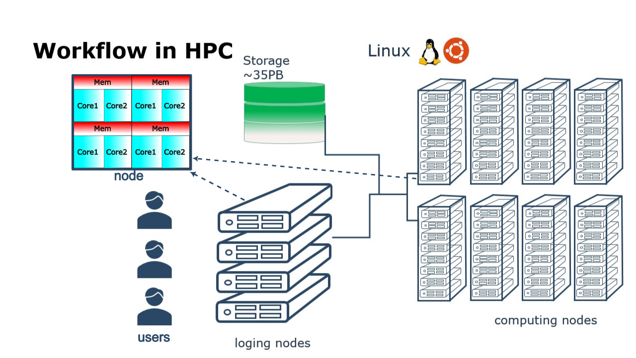
High Performance Computing (HPC) cluster.

Although a serial application can run in such a cluster, it would not gain much of the HPC resources. If fact, one can underuse the cluster if one allocates more resources than what the simulation requires.

Under-using a cluster.

Warning

• Check if the resources that you allocated are being used properly.

• Monitor the usage of hardware resources with tools offered at your HPC center, for instance job-usage at HPC2N.

• Here there are some examples (of many) of what you will need to pay attention when porting a parallel code from your laptop (or another HPC center) to our clusters:

HPC2NUPPMAX/LUNARC/PDC/NSC

We have a tool to monitor the usage of resources called: job-usage at HPC2N.

Parallelizing code in Python

In Python there are different schemes that can be used to parallelize your code. We will only take a look at some of these schemes that illustrate the general concepts of parallel computing. The aim of this lecture is to learn how to run parallel codes in Python rather than learning to write those codes.

Demo

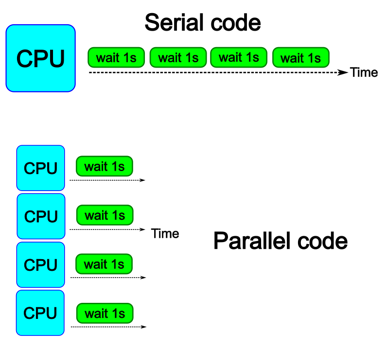
The idea is to parallelize a simple for loop (language-agnostic):

for i start at 1 end at 4
   wait 1 second
end the for loop

The waiting step is used to simulate a task without writing too much code. In this way, one can realize how faster the loop can be executed when threads are added:

In the following example sleep.py the sleep() function is called n times first in serial mode and then by using n processes. To parallelize the serial code we can use the multiprocessing module that is shipped with the base library in Python so that you don’t need to install it.

import sys
from time import perf_counter,sleep
import multiprocessing

# number of iterations
n = 4
# number of processes
numprocesses = 4

def sleep_serial(n):
    for i in range(n):
        sleep(1)


def sleep_threaded(n,numprocesses,processindex):
    # workload for each process
    workload = n/numprocesses
    begin = int(workload*processindex)
    end = int(workload*(processindex+1))
    for i in range(begin,end):
        sleep(1)

if __name__ == "__main__":

    starttime = perf_counter()   # Start timing serial code
    sleep_serial(n)
    endtime = perf_counter()

    print("Time spent serial: %.2f sec" % (endtime-starttime))


    starttime = perf_counter()   # Start timing parallel code
    processes = []
    for i in range(numprocesses):
        p = multiprocessing.Process(target=sleep_threaded, args=(n,numprocesses,i))
        processes.append(p)
        p.start()

    # waiting for the processes
    for p in processes:
        p.join()

    endtime = perf_counter()

    print("Time spent parallel: %.2f sec" % (endtime-starttime))

First load the modules ml GCCcore/11.2.0 Python/3.9.6 (on Kebnekaise) and then run the script with the command srun -A "your-project" -n 1 -c 4 -t 00:05:00 python sleep.py to use 4 processes.

2D integration

The workhorse for this section will be a 2D integration example:

\[\int^{\pi}_{0}\int^{\pi}_{0}\sin(x+y)dxdy = 0\]

One way to perform the integration is by creating a grid in the x and y directions. More specifically, one divides the integration range in both directions into n bins. A serial code (without any optimization) can be seen in the following code block.

integration2d_serial.py

import math
import sys
from time import perf_counter

# grid size
n = 10000

def integration2d_serial(n):
      global integral;
      # interval size (same for X and Y)
      h = math.pi / float(n)
      # cummulative variable
      mysum = 0.0

      # regular integration in the X axis
      for i in range(n):
         x = h * (i + 0.5)
         # regular integration in the Y axis
         for j in range(n):
            y = h * (j + 0.5)
            mysum += math.sin(x + y)

      integral = h**2 * mysum


if __name__ == "__main__":

      starttime = perf_counter()
      integration2d_serial(n)
      endtime = perf_counter()

print("Integral value is %e, Error is %e" % (integral, abs(integral - 0.0)))
print("Time spent: %.2f sec" % (endtime-starttime))

We can run this code on the terminal as follows (similarly at both HPC2N and UPPMAX):

Warning

Although this works on the terminal, having many users doing computations at the same time for this course, could create delays for other users

$ python integration2d_serial.py
Integral value is -7.117752e-17, Error is 7.117752e-17
Time spent: 20.39 sec

Because of that, we can use for short-time jobs the following command:

$ srun -A <your-projec-id> -n 1 -t 00:10:00 python integration2d_serial.py
Integral value is -7.117752e-17, Error is 7.117752e-17
Time spent: 20.39 sec

where srun has the flags that are used in a standard batch file.

Note that outputs can be different, when timing a code a more realistic approach would be to run it several times to get statistics.

One of the crucial steps upon parallelizing a code is identifying its bottlenecks. In the present case, we notice that the most expensive part in this code is the double for loop.

Serial optimizations

Just before we jump into a parallelization project, Python offers some options to make serial code faster. For instance, the Numba module can assist you to obtain a compiled-quality function with minimal efforts. This can be achieved with the njit() decorator:

integration2d_serial_numba.py

from numba import njit
import math
import sys
from time import perf_counter

# grid size
n = 10000

def integration2d_serial(n):
      # interval size (same for X and Y)
      h = math.pi / float(n)
      # cummulative variable
      mysum = 0.0

      # regular integration in the X axis
      for i in range(n):
         x = h * (i + 0.5)
         # regular integration in the Y axis
         for j in range(n):
            y = h * (j + 0.5)
            mysum += math.sin(x + y)

      integral = h**2 * mysum
      return integral


if __name__ == "__main__":

      starttime = perf_counter()
      integral = njit(integration2d_serial)(n)
      endtime = perf_counter()

print("Integral value is %e, Error is %e" % (integral, abs(integral - 0.0)))
print("Time spent: %.2f sec" % (endtime-starttime))

The execution time is now:

$ python integration2d_serial_numba.py
Integral value is -7.117752e-17, Error is 7.117752e-17
Time spent: 1.90 sec

Another option for making serial codes faster, and specially in the case of arithmetic intensive codes, is to write the most expensive parts of them in a compiled language such as Fortran or C/C++. In the next paragraphs we will show you how Fortran code for the 2D integration case can be called in Python.

We start by writing the expensive part of our Python code in a Fortran function in a file called fortran_function.f90:

fortran_function.f90

function integration2d_fortran(n) result(integral)
      implicit none
      integer, parameter :: dp=selected_real_kind(15,9)
      real(kind=dp), parameter   :: pi=3.14159265358979323_dp
      integer, intent(in)        :: n
      real(kind=dp)              :: integral

      integer                    :: i,j
!   interval size
      real(kind=dp)              :: h
!   x and y variables
      real(kind=dp)              :: x,y
!   cummulative variable
      real(kind=dp)              :: mysum

      h = pi/(1.0_dp * n)
      mysum = 0.0_dp
!   regular integration in the X axis
      do i = 0, n-1
         x = h * (i + 0.5_dp)
!      regular integration in the Y axis
         do j = 0, n-1
            y = h * (j + 0.5_dp)
            mysum = mysum + sin(x + y)
         enddo
      enddo

      integral = h*h*mysum

end function integration2d_fortran

Then, we need to compile this code and generate the Python module (myfunction):

Warning

For UPPMAX you may have to change gcc version like:

$ ml gcc/10.3.0

Then continue…

$ f2py -c -m myfunction fortran_function.f90
running build
running config_cc
...

this will produce the Python/C API myfunction.cpython-39-x86_64-linux-gnu.so, which can be called in Python as a module:

call_fortran_code.py

from time import perf_counter
import myfunction
import numpy

# grid size
n = 10000

if __name__ == "__main__":

      starttime = perf_counter()
      integral = myfunction.integration2d_fortran(n)
      endtime = perf_counter()

print("Integral value is %e, Error is %e" % (integral, abs(integral - 0.0)))
print("Time spent: %.2f sec" % (endtime-starttime))

The execution time is considerably reduced:

$ python call_fortran_code.py
Integral value is -7.117752e-17, Error is 7.117752e-17
Time spent: 1.30 sec

Compilation of code can be tedious specially if you are in a developing phase of your code. As an alternative to improve the performance of expensive parts of your code (without using a compiled language) you can write these parts in Julia (which doesn’t require compilation) and then calling Julia code in Python. For the workhorse integration case that we are using, the Julia code can look like this:

julia_function.jl

function integration2d_julia(n::Int)
# interval size
h = π/n
# cummulative variable
mysum = 0.0
# regular integration in the X axis
for i in 0:n-1
   x = h*(i+0.5)
#   regular integration in the Y axis
   for j in 0:n-1
      y = h*(j + 0.5)
      mysum = mysum + sin(x+y)
   end
end
return mysum*h*h
end

A caller script for Julia would be,

call_julia_code.py

Julia v. 1.9.3Julia v. 1.9.4/1.10.4

from time import perf_counter
import julia
from julia import Main

Main.include('julia_function.jl')

# grid size
n = 10000

if __name__ == "__main__":

   starttime = perf_counter()
   integral = Main.integration2d_julia(n)
   endtime = perf_counter()

   print("Integral value is %e, Error is %e" % (integral, abs(integral - 0.0)))
   print("Time spent: %.2f sec" % (endtime-starttime))

Timing in this case is similar to the Fortran serial case:

$ python call_julia_code.py
Integral value is -7.117752e-17, Error is 7.117752e-17
Time spent: 1.29 sec

If even with the previous (and possibly others from your own) serial optimizations your code doesn’t achieve the expected performance, you may start looking for some parallelization scheme. Here, we describe the most common schemes.

Shared Memory

Threads

In a threaded parallelization scheme, the workers (threads) share a global memory address space. The threading module is built into Python so you don’t have to installed it. By using this module, one can create several threads to do some work in parallel (in principle). For jobs dealing with files I/O one can observe some speedup by using the threading module. However, for CPU intensive jobs one would see a decrease in performance w.r.t. the serial code. This is because Python uses the Global Interpreter Lock (GIL) which serializes the code when several threads are used. The GIL serialization is avoided in Python versions > 3.14.

In the following code we used the threading module to parallelize the 2D integration example. Threads are created with the construct threading.Thread(target=function, args=()), where target is the function that will be executed by each thread and args is a tuple containing the arguments of that function. Threads are started with the start() method and when they finish their job they are joined with the join() method,

integration2d_threading.py

import threading
import math
import sys
from time import perf_counter

# grid size
n = 10000
# number of threads
numthreads = 4
# partial sum for each thread
partial_integrals = [None]*numthreads

def integration2d_threading(n,numthreads,threadindex):
      global partial_integrals;
      # interval size (same for X and Y)
      h = math.pi / float(n)
      # cummulative variable
      mysum = 0.0
      # workload for each thread
      workload = n/numthreads
      # lower and upper integration limits for each thread
      begin = int(workload*threadindex)
      end = int(workload*(threadindex+1))
      # regular integration in the X axis
      for i in range(begin,end):
         x = h * (i + 0.5)
         # regular integration in the Y axis
         for j in range(n):
            y = h * (j + 0.5)
            mysum += math.sin(x + y)

      partial_integrals[threadindex] = h**2 * mysum


if __name__ == "__main__":

      starttime = perf_counter()
      # start the threads
      threads = []
      for i in range(numthreads):
         t = threading.Thread(target=integration2d_threading, args=(n,numthreads,i))
         threads.append(t)
         t.start()

      # waiting for the threads
      for t in threads:
         t.join()

      integral = sum(partial_integrals)
      endtime = perf_counter()

print("Integral value is %e, Error is %e" % (integral, abs(integral - 0.0)))
print("Time spent: %.2f sec" % (endtime-starttime))

Notice the output of running this code on the terminal:

$ python integration2d_threading.py
Integral value is 4.492851e-12, Error is 4.492851e-12
Time spent: 21.29 sec

Although we are distributing the work on 4 threads, the execution time is longer than in the serial code. This is due to the GIL mentioned above.

Implicit Threaded

Some libraries like OpenBLAS, LAPACK, and MKL provide an implicit threading mechanism. They are used, for instance, by numpy module for computing linear algebra operations. You can obtain information about the libraries that are available in numpy with numpy.show_config(). This can be useful at the moment of setting the number of threads as these libraries could use different mechanisms for it, for the following example we will use the OpenMP environment variables.

Consider the following code that computes the dot product of a matrix with itself:

dot.py

from time import perf_counter
import numpy as np

A = np.random.rand(3000,3000)
starttime = perf_counter()
B = np.dot(A,A)
endtime = perf_counter()

print("Time spent: %.2f sec" % (endtime-starttime))

the timing for running this code with 1 thread is:

$ export OMP_NUM_THREADS=1
$ python dot.py
Time spent: 1.14 sec

while running with 2 threads is:

$ export OMP_NUM_THREADS=2
$ python dot.py
Time spent: 0.60 sec

It is also possible to use efficient threads if you have blocks of code written in a compiled language. Here, we will see the case of the Fortran code written above where OpenMP threads are used. The parallelized code looks as follows:

fortran_function_openmp.f90

function integration2d_fortran_openmp(n) result(integral)
      !$ use omp_lib
      implicit none
      integer, parameter :: dp=selected_real_kind(15,9)
      real(kind=dp), parameter   :: pi=3.14159265358979323
      integer, intent(in)        :: n
      real(kind=dp)              :: integral

      integer                    :: i,j
!   interval size
      real(kind=dp)              :: h
!   x and y variables
      real(kind=dp)              :: x,y
!   cummulative variable
      real(kind=dp)              :: mysum

      h = pi/(1.0_dp * n)
      mysum = 0.0_dp
!   regular integration in the X axis
!$omp parallel do reduction(+:mysum) private(x,y,j)
      do i = 0, n-1
         x = h * (i + 0.5_dp)
!      regular integration in the Y axis
         do j = 0, n-1
            y = h * (j + 0.5_dp)
            mysum = mysum + sin(x + y)
         enddo
      enddo
!$omp end parallel do

      integral = h*h*mysum

end function integration2d_fortran_openmp

The way to compile this code differs to the one we saw before, now we will need the flags for OpenMP:

$ f2py -c --f90flags='-fopenmp' -lgomp -m myfunction_openmp fortran_function_openmp.f90

the generated module can be then loaded,

call_fortran_code_openmp.py

from time import perf_counter
import myfunction_openmp
import numpy

# grid size
n = 10000

if __name__ == "__main__":

      starttime = perf_counter()
      integral = myfunction_openmp.integration2d_fortran_openmp(n)
      endtime = perf_counter()

      print("Integral value is %e, Error is %e" % (integral, abs(integral - 0.0)))
      print("Time spent: %.2f sec" % (endtime-starttime))

the execution time by using 4 threads is:

$ export OMP_NUM_THREADS=4
$ srun -A projID -t 00:08:00 -o output_%j.out -e error_%j.err -c 4 python call_fortran_code_openmp.py
Integral value is 4.492945e-12, Error is 4.492945e-12
Time spent: 0.37 sec

More information about how OpenMP works can be found in the material of a previous OpenMP course offered by some of us.

PyOMP

The PyOMP module offers an interface for writing OpenMP directives in Python, so the compilation step mentioned above is avoided. PyOMP is an extension of Numba.

integration2d_omp.py

import math
from time import perf_counter
from numba.openmp import njit
from numba.openmp import openmp_context as openmp

# grid size
n = 100000

@njit
def integration2d_omp(n):
   h = math.pi / float(n)
   mysum = 0.0

   # parallelize the outer loop
   with openmp("parallel for reduction(+:mysum)"):
      for i in range(n):
            x = h * (i + 0.5)
            for j in range(n):
               y = h * (j + 0.5)
               mysum += math.sin(x + y)

   return h**2 * mysum


if __name__ == "__main__":
   start = perf_counter()
   integral = integration2d_omp(n)
   end = perf_counter()

   print(f"Integral value is {integral:e}, Error is {abs(integral - 0.0):e}")
   print(f"Time spent: {end - start:.2f} sec")

$ export OMP_NUM_THREADS=1
$ srun -A projID -t 00:08:00 -o output_%j.out -e error_%j.err -c 1 python integration2d_omp.py
Integral value is 1.969642e-16, Error is 1.969642e-16
Time spent: 120.26 sec

$ export OMP_NUM_THREADS=4
$ srun -A projID -t 00:08:00 -o output_%j.out -e error_%j.err -c 4 python integration2d_omp.py
Integral value is 1.353859e-10, Error is 1.353859e-10
Time spent: 36.11 sec

Distributed Memory

Distributed

In the distributed parallelization scheme the workers (processes) can share some common memory but they can also exchange information by sending and receiving messages for instance.

integration2d_multiprocessing.py

import multiprocessing
from multiprocessing import Array
import math
import sys
from time import perf_counter

# grid size
n = 10000
# number of processes
numprocesses = 4
# partial sum for each thread
partial_integrals = Array('d',[0]*numprocesses, lock=False)

def integration2d_multiprocessing(n,numprocesses,processindex):
      global partial_integrals;
      # interval size (same for X and Y)
      h = math.pi / float(n)
      # cummulative variable
      mysum = 0.0
      # workload for each process
      workload = n/numprocesses

      begin = int(workload*processindex)
      end = int(workload*(processindex+1))
      # regular integration in the X axis
      for i in range(begin,end):
         x = h * (i + 0.5)
         # regular integration in the Y axis
         for j in range(n):
            y = h * (j + 0.5)
            mysum += math.sin(x + y)

      partial_integrals[processindex] = h**2 * mysum


if __name__ == "__main__":

      starttime = perf_counter()

      processes = []
      for i in range(numprocesses):
         p = multiprocessing.Process(target=integration2d_multiprocessing, args=(n,numprocesses,i))
         processes.append(p)
         p.start()

      # waiting for the processes
      for p in processes:
         p.join()

      integral = sum(partial_integrals)
      endtime = perf_counter()

      print("Integral value is %e, Error is %e" % (integral, abs(integral - 0.0)))
      print("Time spent: %.2f sec" % (endtime-starttime))

In this case, the execution time is reduced:

$ python integration2d_multiprocessing.py
Integral value is 4.492851e-12, Error is 4.492851e-12
Time spent: 6.06 sec

MPI

More details for the MPI parallelization scheme in Python can be found in a previous MPI course offered by some of us.

integration2d_mpi.py

from mpi4py import MPI
import math
import sys
from time import perf_counter

# MPI communicator
comm = MPI.COMM_WORLD
# MPI size of communicator
numprocs = comm.Get_size()
# MPI rank of each process
myrank = comm.Get_rank()

# grid size
n = 10000

def integration2d_mpi(n,numprocs,myrank):
      # interval size (same for X and Y)
      h = math.pi / float(n)
      # cummulative variable
      mysum = 0.0
      # workload for each process
      workload = n/numprocs

      begin = int(workload*myrank)
      end = int(workload*(myrank+1))
      # regular integration in the X axis
      for i in range(begin,end):
         x = h * (i + 0.5)
         # regular integration in the Y axis
         for j in range(n):
            y = h * (j + 0.5)
            mysum += math.sin(x + y)

      partial_integrals = h**2 * mysum
      return partial_integrals


if __name__ == "__main__":

      starttime = perf_counter()

      p = integration2d_mpi(n,numprocs,myrank)

      # MPI reduction
      integral = comm.reduce(p, op=MPI.SUM, root=0)

      endtime = perf_counter()

      if myrank == 0:
         print("Integral value is %e, Error is %e" % (integral, abs(integral - 0.0)))
         print("Time spent: %.2f sec" % (endtime-starttime))

Execution of this code gives the following output:

$ mpirun -np 4 python integration2d_mpi.py
Integral value is 4.492851e-12, Error is 4.492851e-12
Time spent: 5.76 sec

For long jobs, one will need to run in batch mode. Here is an example of a batch script for this MPI example,

HPC2NUPPMAXNSCLUNARCPDC

#!/bin/bash
#SBATCH -A hpc2n20XX-XYZ
#SBATCH -t 00:05:00        # wall time
#SBATCH -n 4
#SBATCH -o output_%j.out   # output file
#SBATCH -e error_%j.err    # error messages

ml purge > /dev/null 2>&1
ml GCCcore/11.2.0 Python/3.9.6
ml GCC/11.2.0 OpenMPI/4.1.1
#ml Julia/1.7.1-linux-x86_64  # if Julia is needed

source /proj/nobackup/<your-project-storage>/vpyenv-python-course/bin/activate

mpirun -np 4 python integration2d_mpi.py

Heat (advanced)

Heat is a library for distributing tensor operations by using MPI as a backend. Heat uses Distributed N-Dimensional (DND) arrays that can be seen as a global array. Locally, each rank retains a chunk of the array which is a tensor PyTorch tensor:

heat_datatypes.py

import heat as ht

x = ht.arange(10, split=0)

print(type(x))        # <class 'heat.core.dndarray.DNDarray'>
print(type(x.larray)) # <class 'torch.Tensor'>

$ srun -A projectID -t 00:08:00 -o output_%j.out -e error_%j.err -n 2 python heat_datatypes.py

Output:
   <class 'heat.core.dndarray.DNDarray'>
   <class 'torch.Tensor'>
   <class 'heat.core.dndarray.DNDarray'>
   <class 'torch.Tensor'>

More details for this package can be found here Heat package.

Example 1: Distributing matrix-matrix multiplication operations

heat_matmat.py

import heat as ht
import torch
import time

if torch.cuda.is_available():
   device = "gpu"
else:
   device = "cpu"

# load large matrices distributed across CPUs/GPUs
A = ht.random.randn(10000, 10000, split=0, device=device)  # Split along rows
B = ht.random.randn(10000, 10000, split=None, device=device)  # Do not split just copy

# Perform distributed matrix multiplication
start = time.time()
C = ht.linalg.matmul(A, B)
end = time.time()
print("rank= ", ht.MPI_WORLD.rank, "reported time= ",  end-start)

Example 2: Distributing gradients

heat_gradients.py

import heat as ht
import torch
import torch.nn as nn
import torch.optim as optim
import time

# Distributed dataset
X = ht.random.randn(30000, 10000, split=0)
y = ht.random.randn(30000, 1, split=0)

# Local model per rank
model = nn.Linear(10000, 1)
optimizer = optim.SGD(model.parameters(), lr=0.01)

start = time.time()
# Train local arrays
for epoch in range(1000):
   out = model(X.larray)
   loss = torch.mean((out - y.larray) ** 2)
   optimizer.zero_grad()
   loss.backward()
   optimizer.step()

   # Average parameters across ranks (distributed synchronization)
   for param in model.parameters():
      ht.MPI_WORLD.Allreduce(ht.communication.MPI.IN_PLACE, param.data, op=ht.communication.MPI.SUM)
      param.data /= ht.MPI_WORLD.size

end = time.time()
print("rank= ", ht.MPI_WORLD.rank, "reported time= ",  end-start)
print(f"Rank {ht.MPI_WORLD.rank} done training")

Monitoring resources’ usage

Monitoring the resources that a certain job uses is important specially when this job is expected to run on many CPUs and/or GPUs. It could happen, for instance, that an incorrect module is loaded or the command for running on many CPUs is not the proper one and our job runs in serial mode while we allocated possibly many CPUs/GPUs. For this reason, there are several tools available in our centers to monitor the performance of running jobs.

HPC2N

On a Kebnekaise terminal, you can type the command:

$ job-usage job_ID

where job_ID is the number obtained when you submit your job with the sbatch command. This will give you a URL that you can copy and then paste in your local browser. The results can be seen in a graphical manner a couple of minutes after the job starts running, here there is one example of how this looks like:

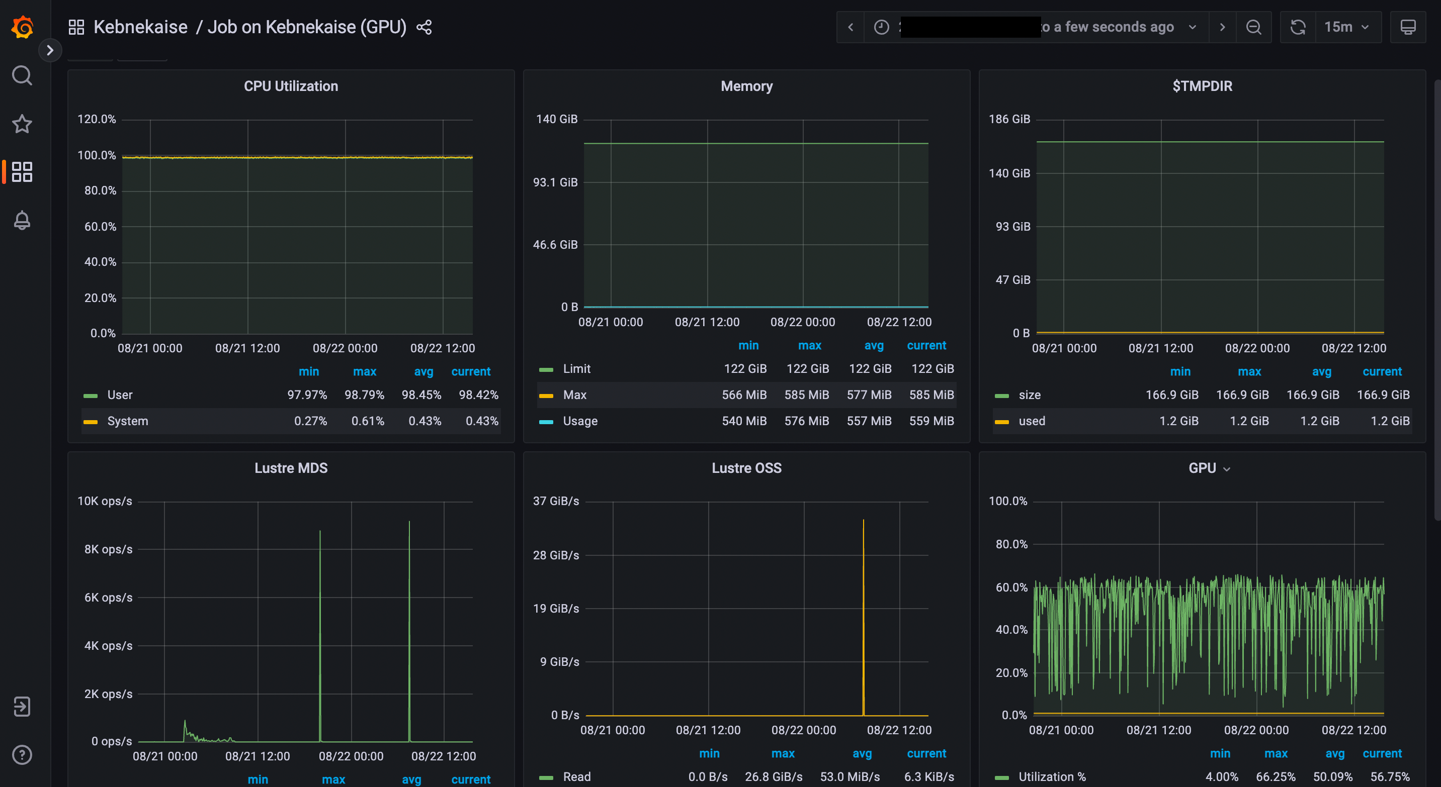
The resources used by a job can be monitored in your local browser. For this job, we can notice that 100% of the requested CPU and 60% of the GPU resources are being used.

Exercises

Running a parallel code efficiently

In this exercise we will run a parallelized code that performs a 2D integration:

\[\int^{\pi}_{0}\int^{\pi}_{0}\sin(x+y)dxdy = 0\]

One way to perform the integration is by creating a grid in the x and y directions. More specifically, one divides the integration range in both directions into n bins.

Here is a parallel code using the multiprocessing module in Python (call it integration2d_multiprocessing.py):

integration2d_multiprocessing.py

import multiprocessing
from multiprocessing import Array
import math
import sys
from time import perf_counter

# grid size
n = 5000
# number of processes
numprocesses = *FIXME*
# partial sum for each thread
partial_integrals = Array('d',[0]*numprocesses, lock=False)

# Implementation of the 2D integration function (non-optimal implementation)
def integration2d_multiprocessing(n,numprocesses,processindex):
   global partial_integrals;
   # interval size (same for X and Y)
   h = math.pi / float(n)
   # cummulative variable
   mysum = 0.0
   # workload for each process
   workload = n/numprocesses

   begin = int(workload*processindex)
   end = int(workload*(processindex+1))
   # regular integration in the X axis
   for i in range(begin,end):
      x = h * (i + 0.5)
      # regular integration in the Y axis
      for j in range(n):
            y = h * (j + 0.5)
            mysum += math.sin(x + y)

   partial_integrals[processindex] = h**2 * mysum


if __name__ == "__main__":

   starttime = perf_counter()

   processes = []
   for i in range(numprocesses):
      p = multiprocessing.Process(target=integration2d_multiprocessing, args=(n,numprocesses,i))
      processes.append(p)
      p.start()

   # waiting for the processes
   for p in processes:
      p.join()

   integral = sum(partial_integrals)
   endtime = perf_counter()

print("Integral value is %e, Error is %e" % (integral, abs(integral - 0.0)))
print("Time spent: %.2f sec" % (endtime-starttime))

Run the code with the following batch script.

job.sh

UPPMAXHPC2NLUNARCNSCPDC

#!/bin/bash -l
#SBATCH -A naiss202X-XY-XYZ     # your project_ID
#SBATCH -J job-serial           # name of the job
#SBATCH -n *FIXME*              # nr. tasks/coresw
#SBATCH --time=00:20:00         # requested time
#SBATCH --error=job.%J.err      # error file
#SBATCH --output=job.%J.out     # output file

# Load any modules you need, here for Python 3.11.8 and compatible SciPy-bundle
module load python/3.11.8
python integration2d_multiprocessing.py

Try different number of cores for this batch script (FIXME string) using the sequence: 1,2,4,8,12, and 14. Note: this number should match the number of processes (also a FIXME string) in the Python script. Collect the timings that are printed out in the job.*.out. According to these execution times what would be the number of cores that gives the optimal (fastest) simulation?

Challenge: Increase the grid size (n) to 15000 and submit the batch job with 4 workers (in the Python script) and request 5 cores in the batch script. Monitor the usage of resources with tools available at your center, for instance top (UPPMAX) or job-usage (HPC2N).

Parallelizing a for loop workflow (Advanced)

Create a Data Frame containing two features, one called ID which has integer values from 1 to 10000, and the other called Value that contains 10000 integers starting from 3 and goes in steps of 2 (3, 5, 7, …). The following codes contain parallelized workflows whose goal is to compute the average of the whole feature Value using some number of workers. Substitute the FIXME strings in the following codes to perform the tasks given in the comments.

The main idea for all languages is to divide the workload across all workers. You can run the codes as suggested for each language.

Pandas is available in the following combo ml GCC/12.3.0 SciPy-bundle/2023.07 (HPC2N) and ml python/3.11.8 (UPPMAX). Call the script script-df.py.

import pandas as pd
import multiprocessing

# Create a DataFrame with two sets of values ID and Value
data_df = pd.DataFrame({
   'ID': range(1, 10001),
   'Value': range(3, 20002, 2)  # Generate 10000 odd numbers starting from 3
})

# Define a function to calculate the sum of a vector
def calculate_sum(values):
   total_sum = *FIXME*(values)
   return *FIXME*

# Split the 'Value' column into chunks of size 1000
chunk_size = *FIXME*
value_chunks = [data_df['Value'][*FIXME*:*FIXME*] for i in range(0, len(data_df['*FIXME*']), *FIXME*)]

# Create a Pool of 4 worker processes, this is required by multiprocessing
pool = multiprocessing.Pool(processes=*FIXME*)

# Map the calculate_sum function to each chunk of data in parallel
results = pool.map(*FIXME: function*, *FIXME: chunk size*)

# Close the pool to free up resources, if the pool won't be used further
pool.close()

# Combine the partial results to get the total sum
total_sum = sum(results)

# Compute the mean by dividing the total sum by the total length of the column 'Value'
mean_value = *FIXME* / len(data_df['*FIXME*'])

# Print the mean value
print(mean_value)

Run the code with the batch script:

UPPMAXHPC2NLUNARCNSCPDC

#!/bin/bash -l
#SBATCH -A naiss202u-w-xyz  # your project_ID
#SBATCH -J job-parallel      # name of the job
#SBATCH -n 4                 # nr. tasks/coresw
#SBATCH --time=00:20:00      # requested time
#SBATCH --error=job.%J.err   # error file
#SBATCH --output=job.%J.out  # output file

# Load any modules you need, here for Python 3.11.8 and compatible SciPy-bundle
module load python/3.11.8
python script-df.py

Solution

import pandas as pd
import multiprocessing

# Create a DataFrame with two sets of values ID and Value
data_df = pd.DataFrame({
   'ID': range(1, 10001),
   'Value': range(3, 20002, 2)  # Generate 10000 odd numbers starting from 3
})

# Define a function to calculate the sum of a vector
def calculate_sum(values):
   total_sum = sum(values)
   return total_sum

# Split the 'Value' column into chunks
chunk_size = 1000
value_chunks = [data_df['Value'][i:i+chunk_size] for i in range(0, len(data_df['Value']), chunk_size)]

# Create a Pool of 4 worker processes, this is required by multiprocessing
pool = multiprocessing.Pool(processes=4)

# Map the calculate_sum function to each chunk of data in parallel
results = pool.map(calculate_sum, value_chunks)

# Close the pool to free up resources, if the pool won't be used further
pool.close()

# Combine the partial results to get the total sum
total_sum = sum(results)

# Compute the mean by dividing the total sum by the total length of the column 'Value'
mean_value = total_sum / len(data_df['Value'])

# Print the mean value
print(mean_value)

See also

• On parallel software engineering education using python

• List of parallel libraries for Python

• Wikipedias’ article on Parallel Computing

• The book High Performance Python is a good resource for ways of speeding up Python code.

Keypoints

• You deploy cores and nodes via SLURM, either in interactive mode or batch

• In Python, threads, distributed and MPI parallelization can be used.