Dimensionality Reduction
Guest Lecture by Professor Anders Hast
Distinguished University Teacher, InfraVis, UU Node
Research page: andershast.com
email: anders.hast@it.uu.se
InfraVis: infravis.se
Questions
How and why dimensionality reduction is an important tool?
Objectives
We will look at tools for visualising what cannot easily be seen, i.e. high dimensionality reduction
Share insights and experience from Anders’s own research
visualisation <–> Science
Clustering
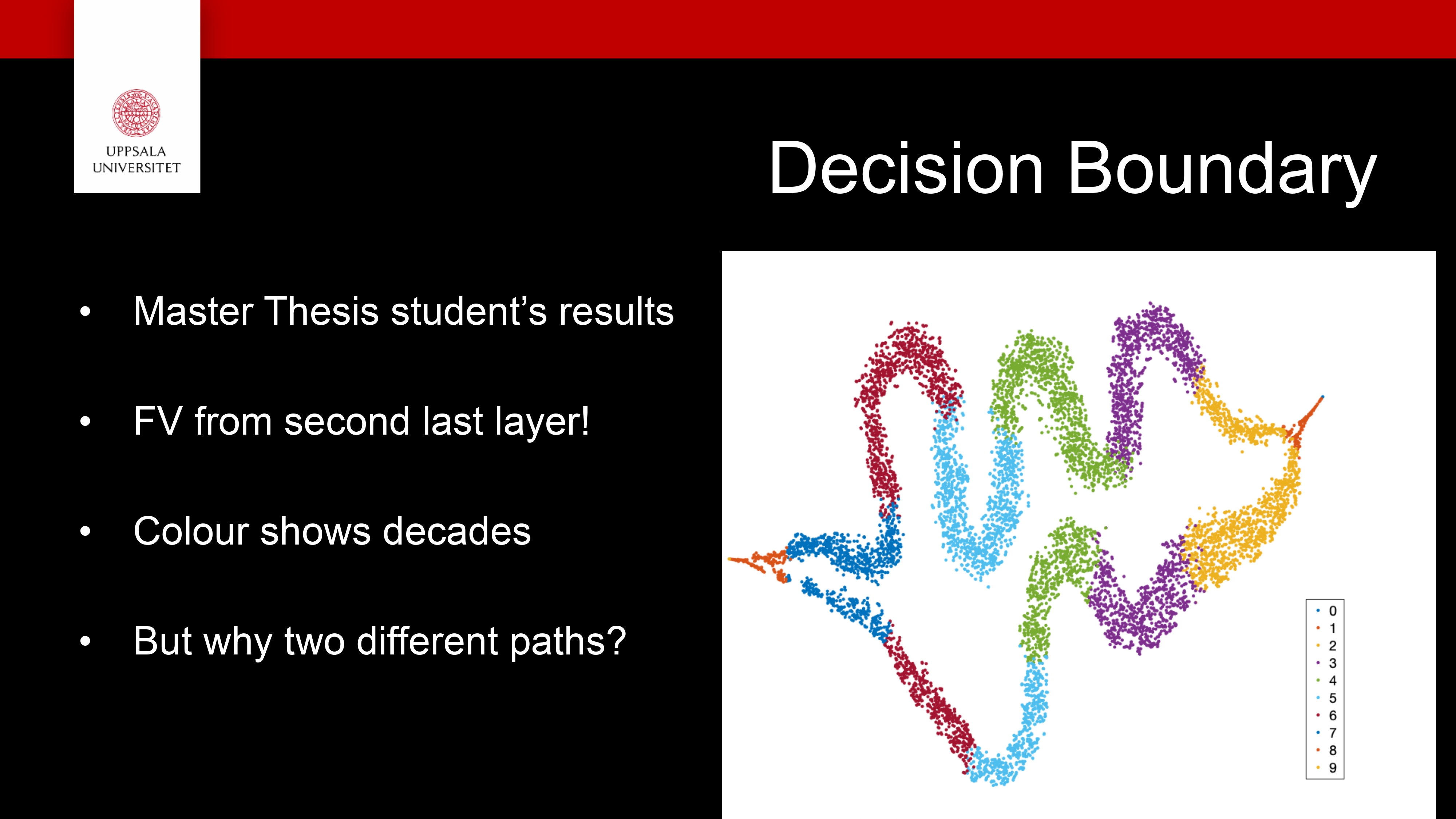
Decision boundary
We will look at tools for visualising what cannot easily be seen, i.e. high dimensionality reduction
We will also see that you can make discoveries in your visualisations!
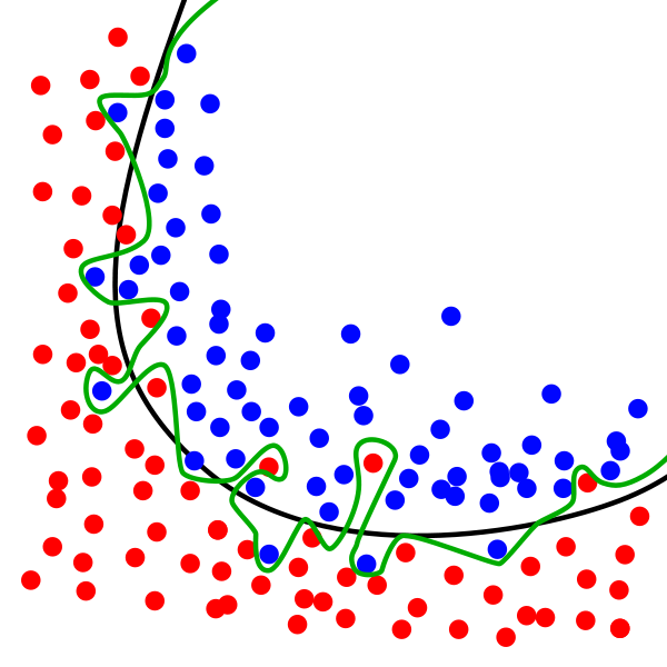
What is a typical machine learning task?
Differ between different classes of features
Features usually have more than 3 dimensions, hundreds or even thousands!
The idea is to find a separating curve in high dimensional space
Usually we visualise this in 2D since it is easier to understand!
We will look at several techniques to do this!
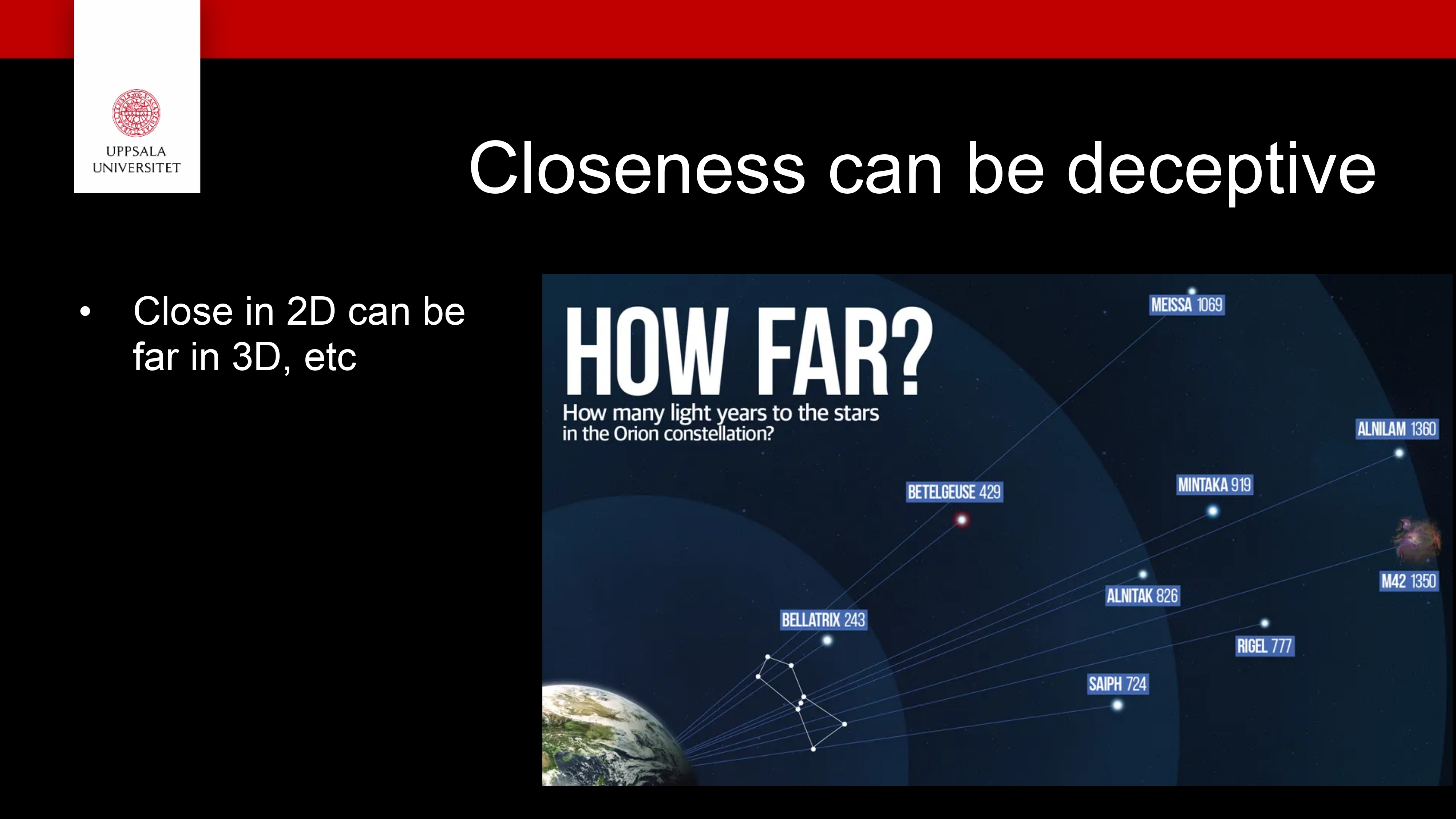
If we can separate in 2D it can often be done in High dimensional space and vice versa!
Dimensionality reduction:
Project from several dimensions to fewer, often 2D or 3D
Remember: we get a distorted picture of the high dimensional space!
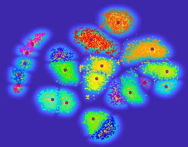
- Some techniques
SOM
PCA
t-SNE
UMAP

Some Dimensionality Reduction Techniques:
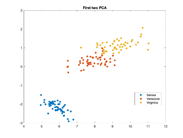
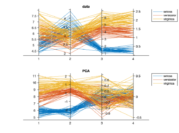
PCA (on Iris Data)
PCA = “find the directions where the data varies the most.”
PCA finds a new coordinate system that fits the data:
The first axis (1st principal component) points where the data spreads out the most.
The second axis (2nd principal component) is perpendicular to the first and captures the next largest spread.
The eigenvectors are the directions of those new axes — the principal components.
The eigenvalues tell you how much variance (spread) each component captures.
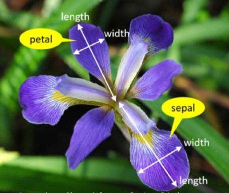
Fisher’s iris data consists of measurements on the sepal length, sepal width, petal length, and petal width for 150 iris specimens.
There are 50 specimens from each of three species.
One axis per data element (which ones are discriminant?)
Follow each individual using the lines
Iris and its PCA
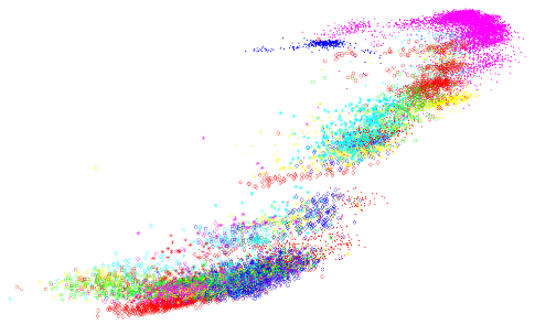
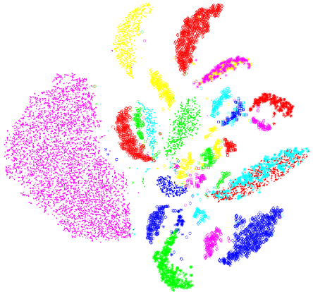
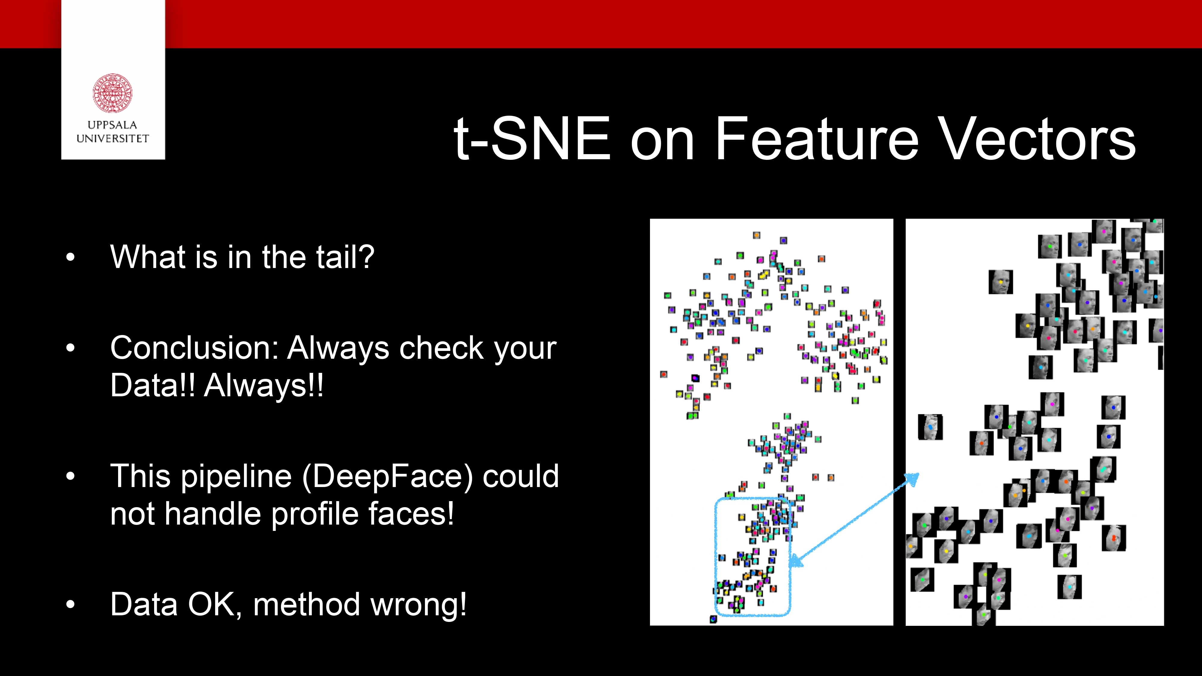
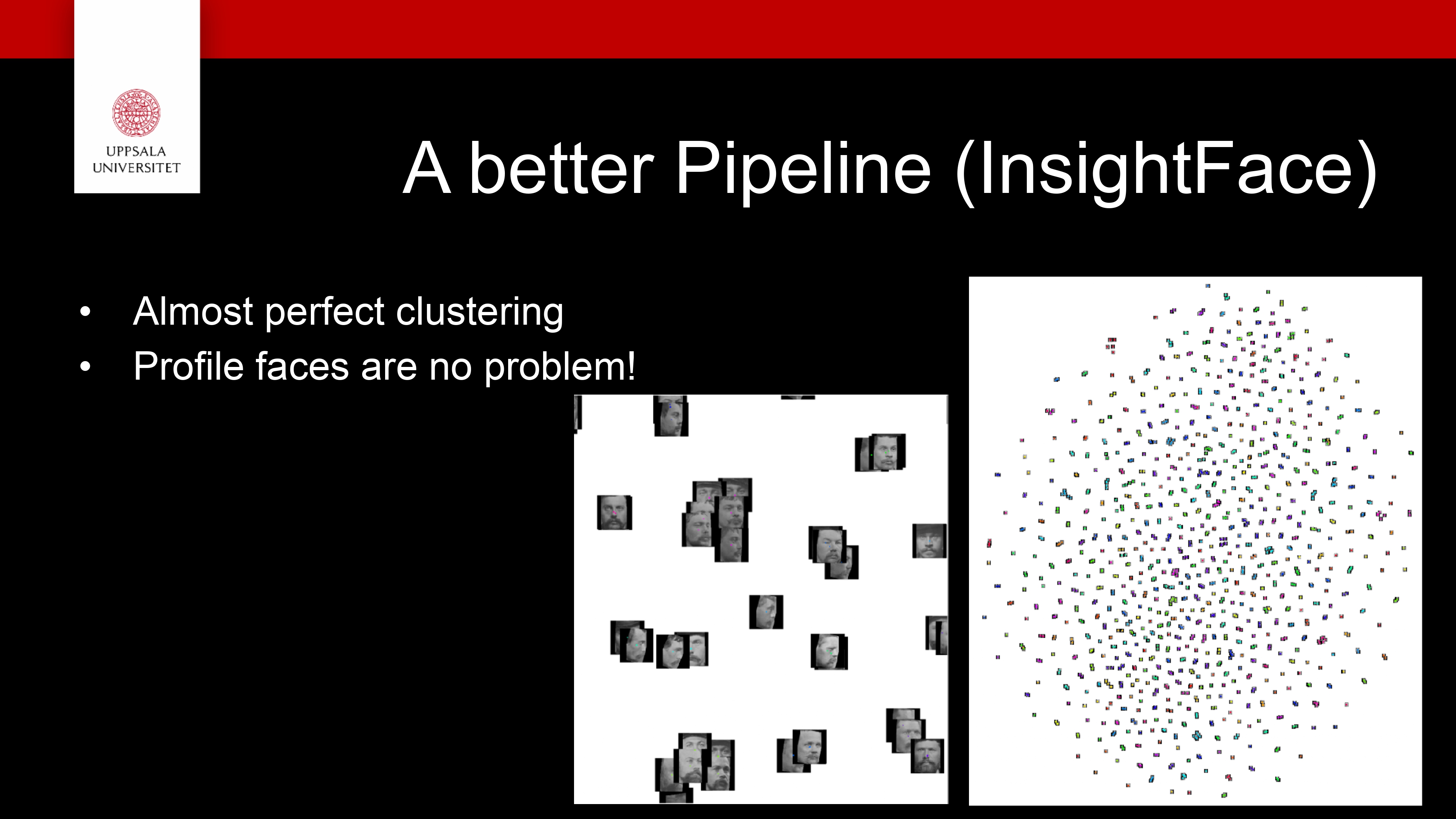
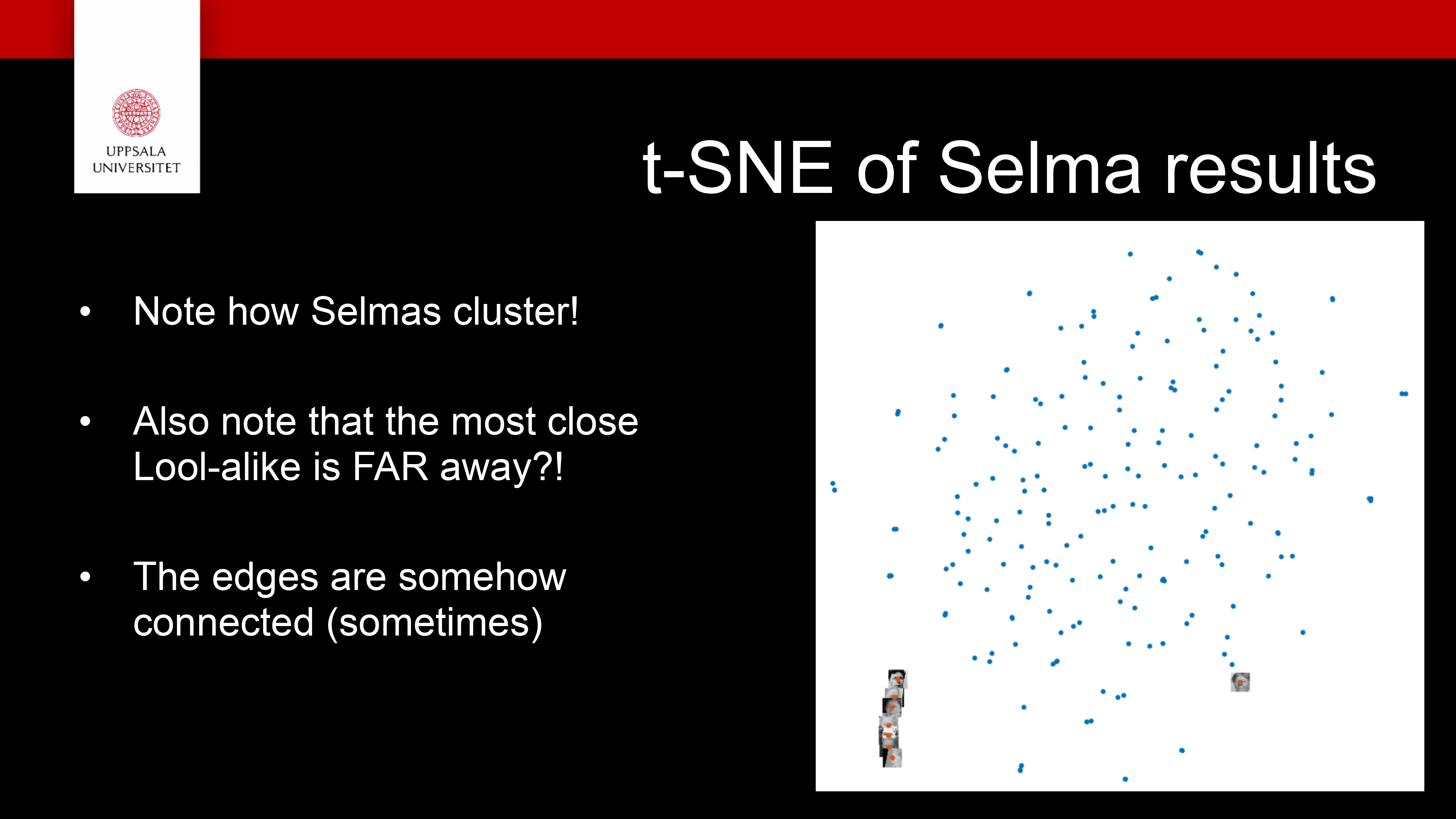
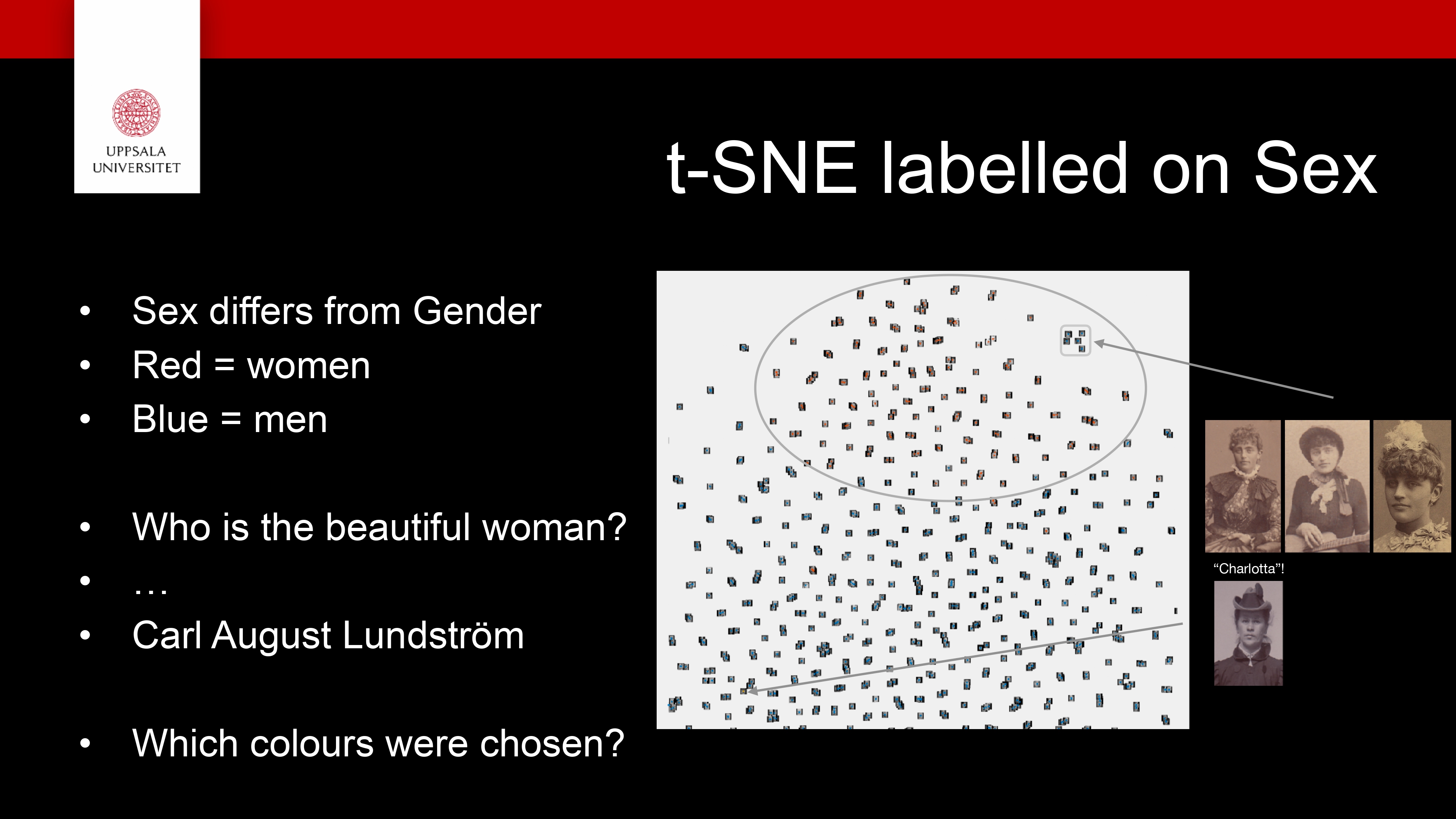
t-SNE
A dimensionality-reduction method for visualising high- dimensional data in 2D or 3D
It keeps similar points close together and dissimilar ones far apart
Works by turning distances between points into probabilities of being neighbours, both in the original space and in the low-dimensional map
Then it moves points to make those probabilities match (minimizing KL divergence)
Uses a Student’s t-distribution in 2D to keep clusters separated and avoid crowding
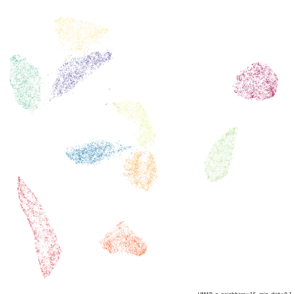
UMAP
A nonlinear dimensionality-reduction method, like t-SNE, used to visualize high-dimensional data in 2D or 3D
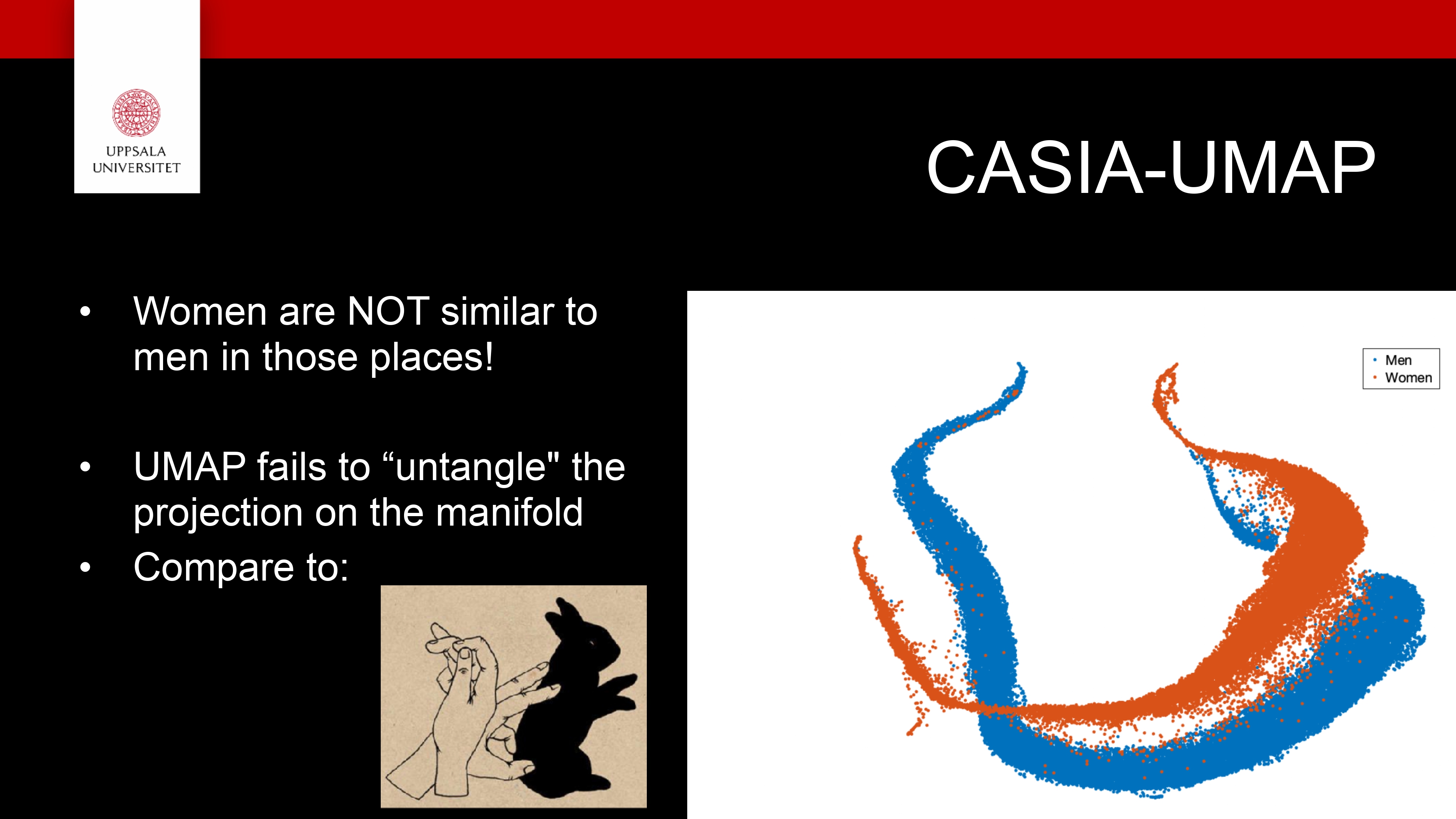
Based on manifold theory — it assumes your data lies on a curved surface within a high-dimensional space
Builds a graph of local relationships (who’s close to whom) in the original space, then finds a low-dimensional layout that preserves those relationships
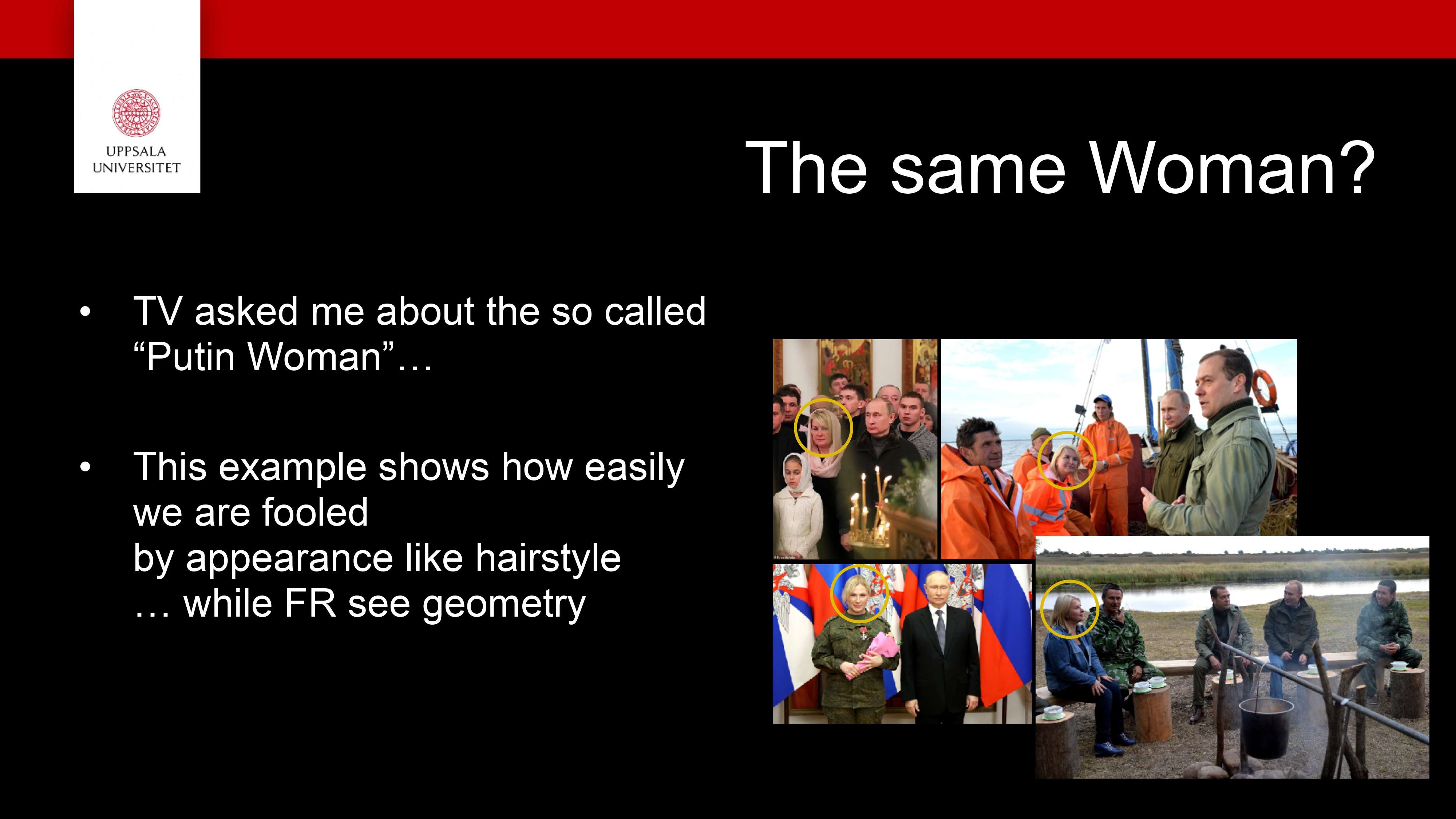
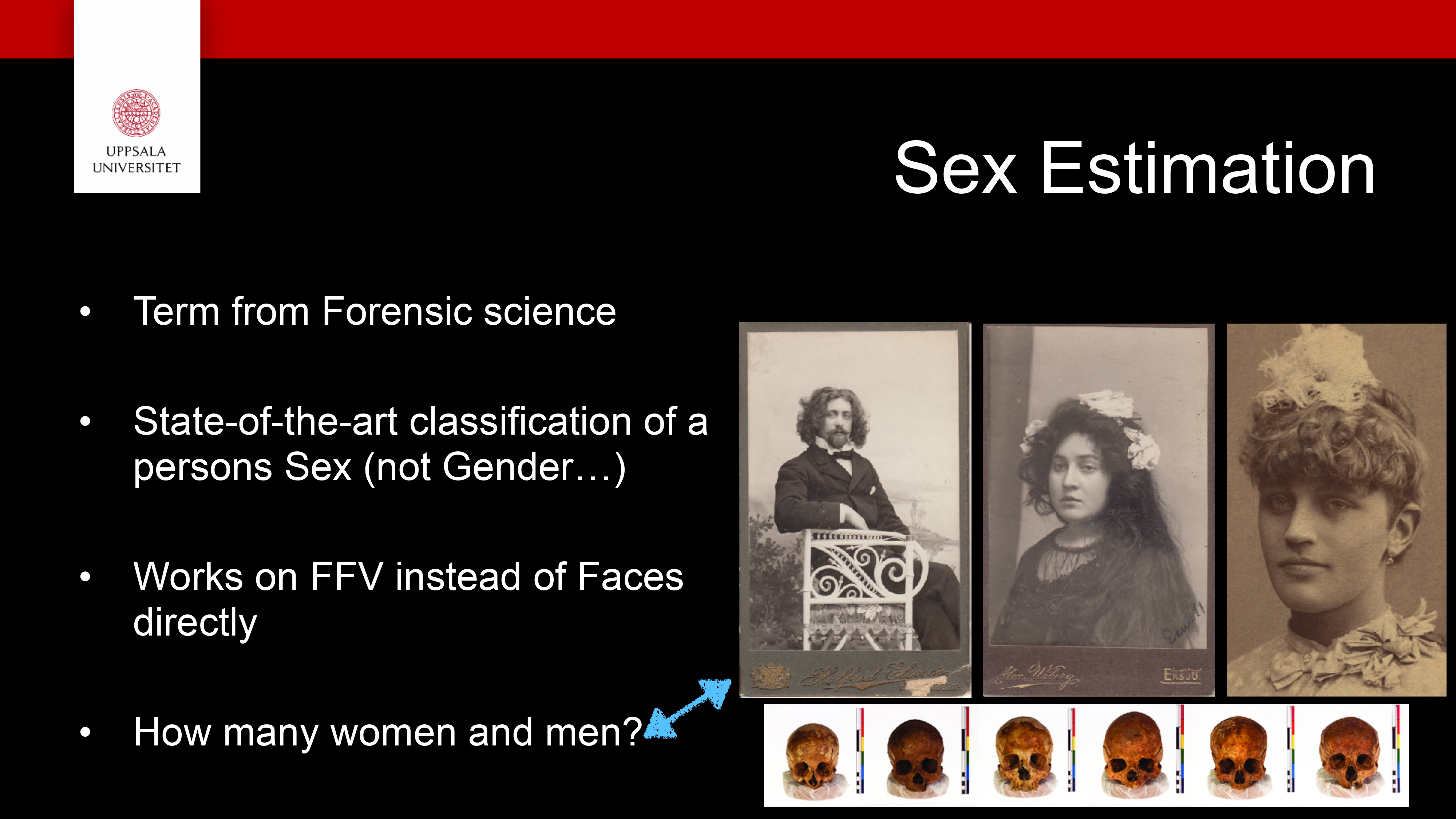
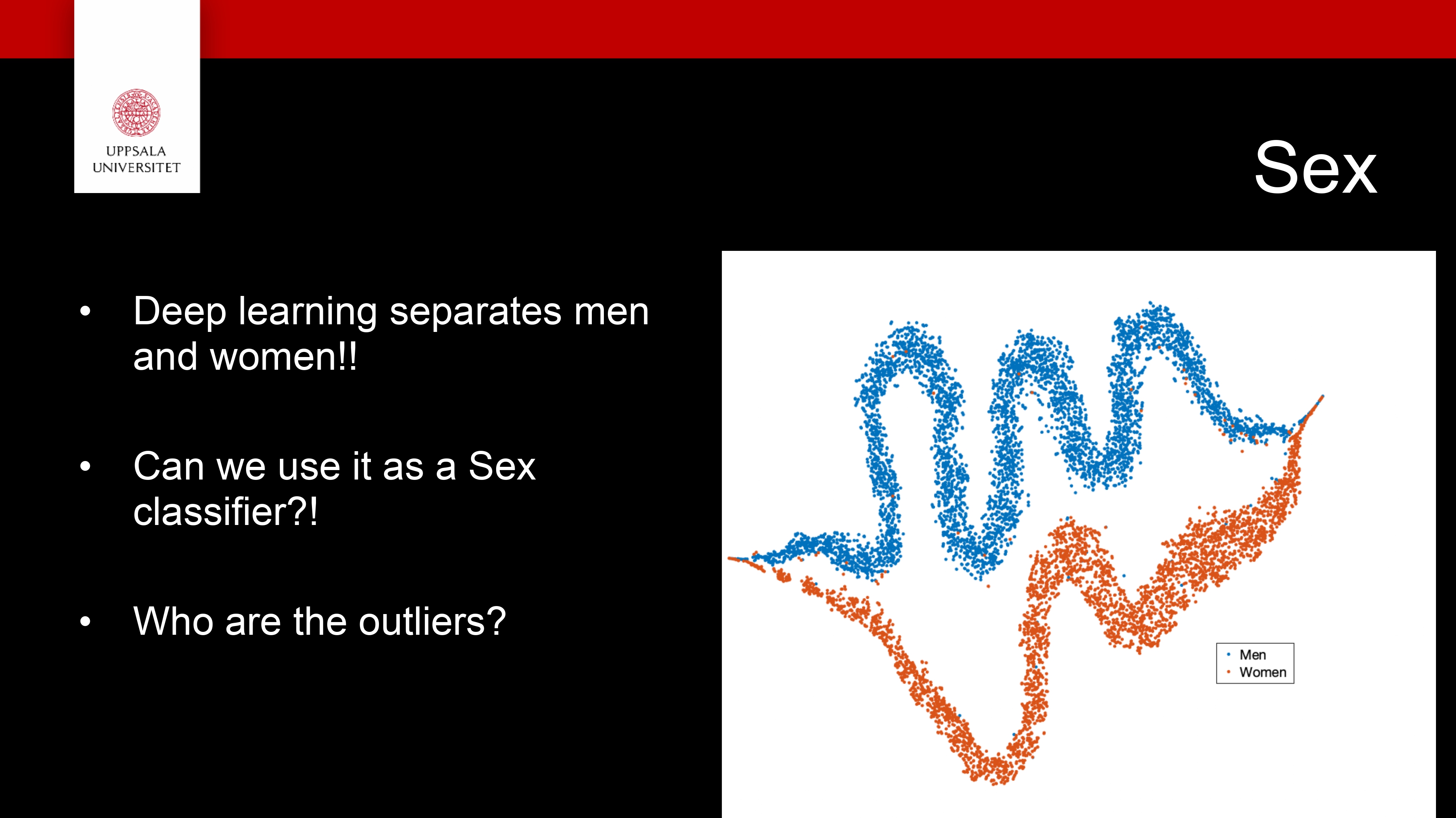
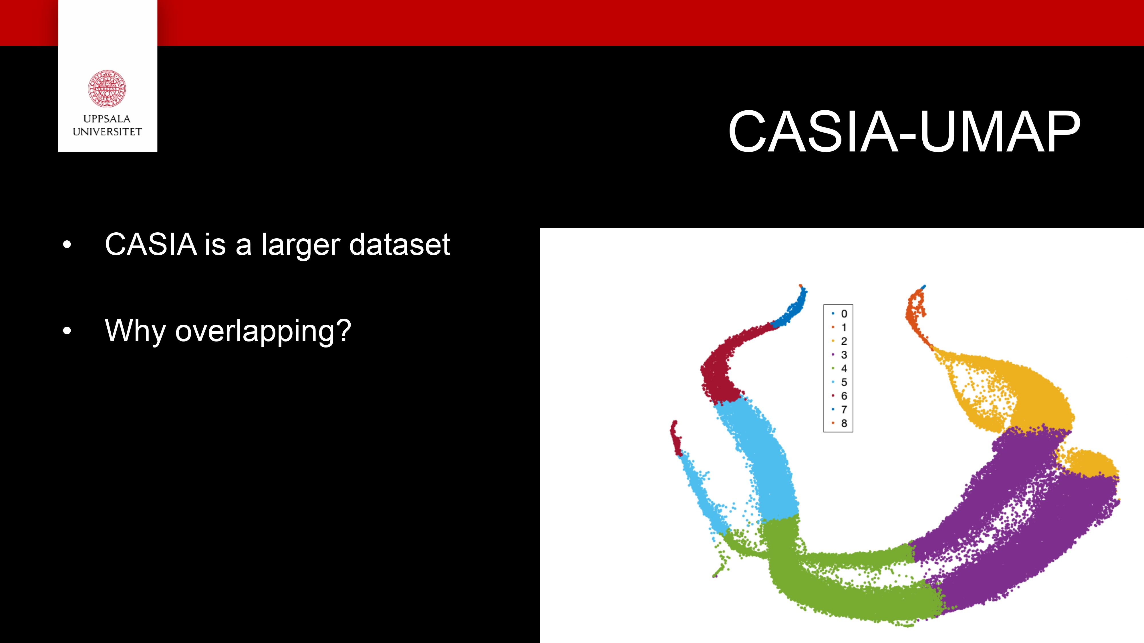
Face Recognition (FR) Use case
InfraVis slides on FR
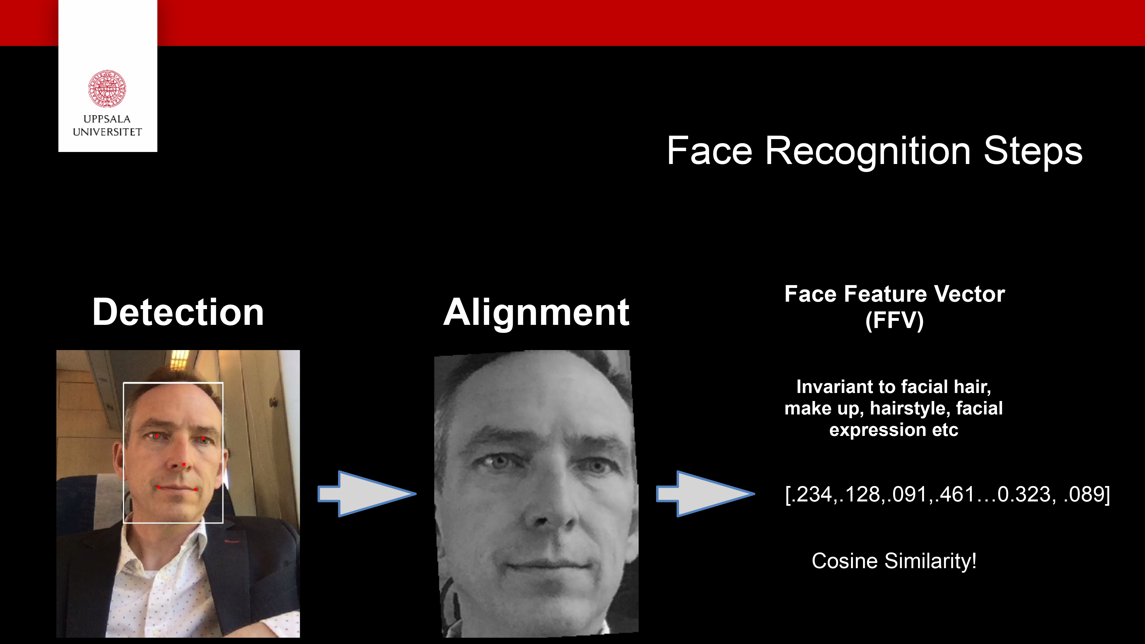
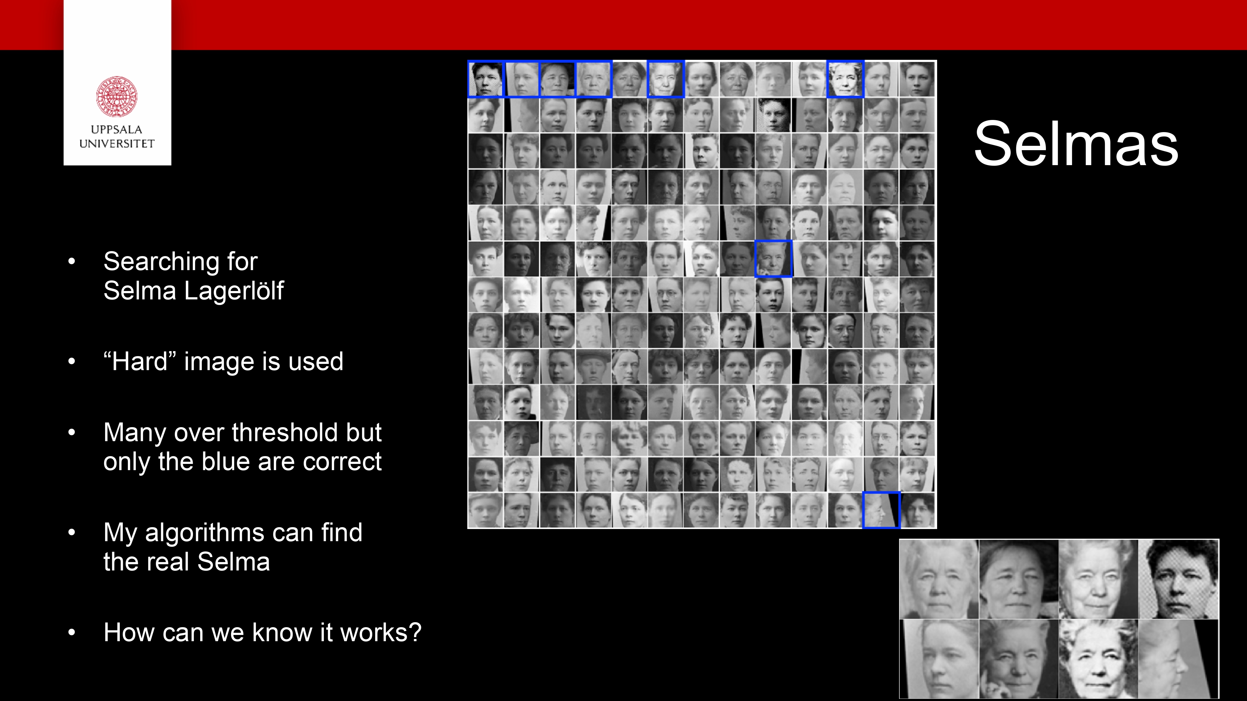
Keypoints
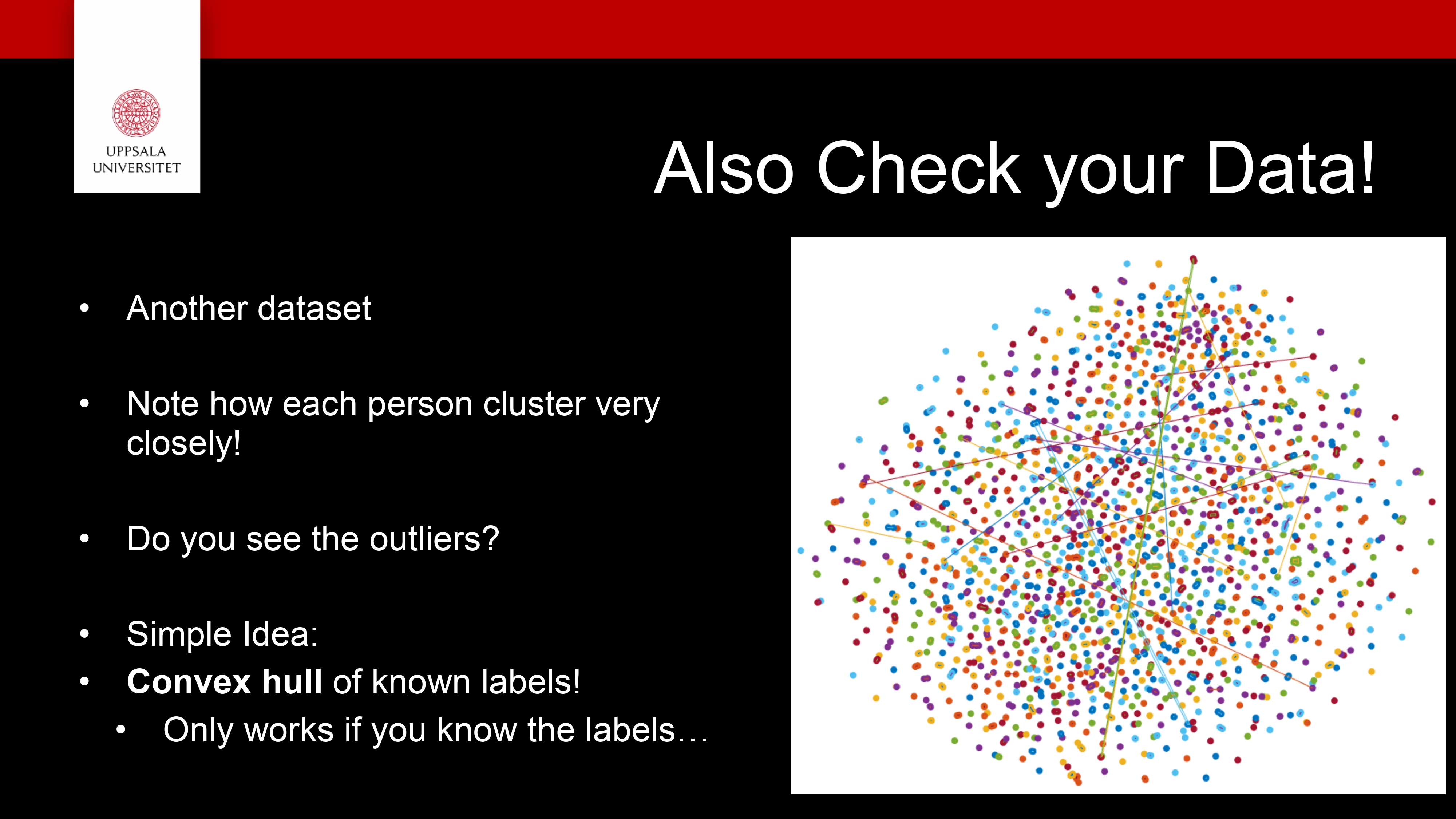
We looked at several dimensionality reduction techniques
They are useful to be able to explore your high dimensional data!
- But not only nice pictures
Make discoveries!
New results!
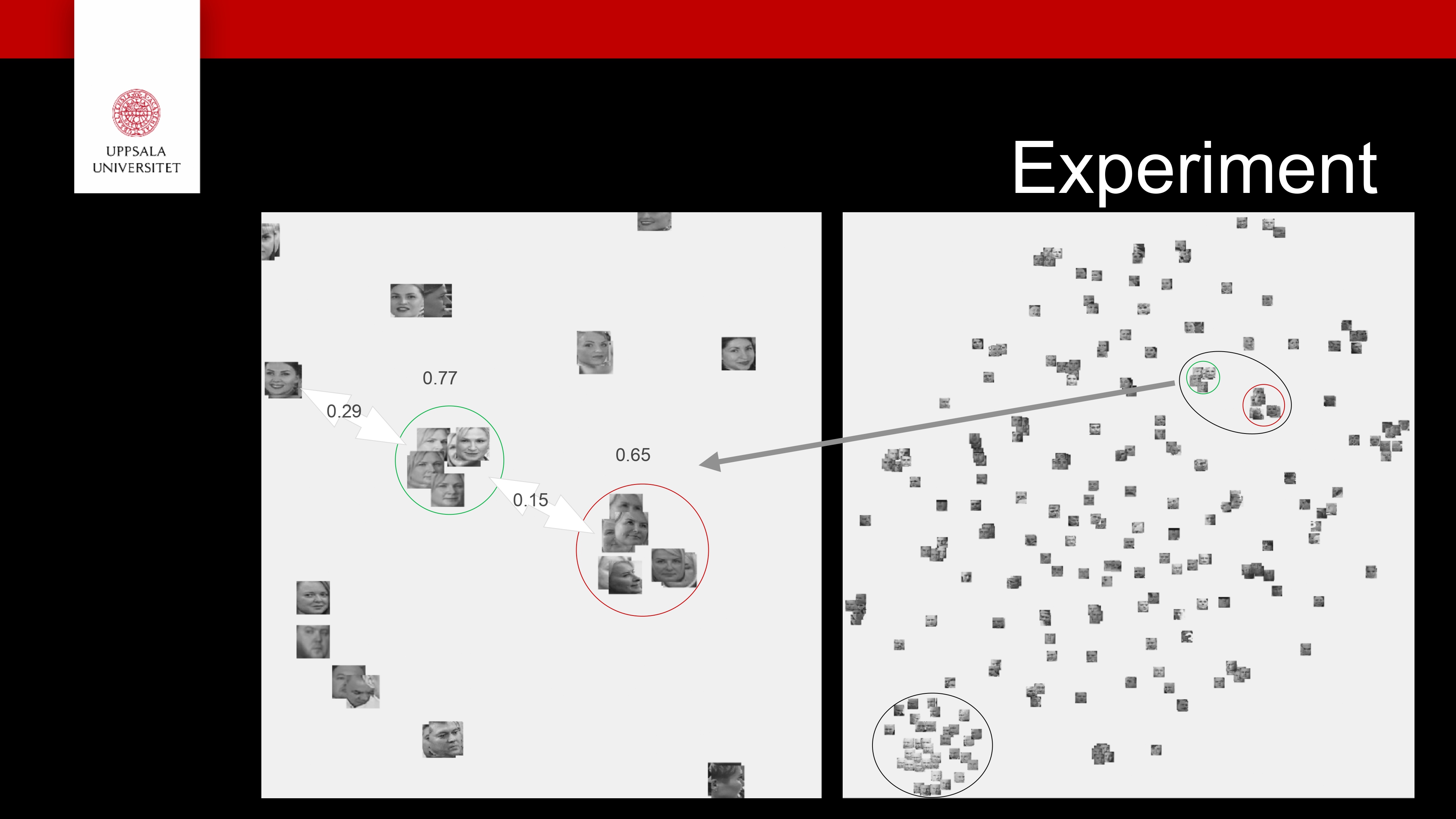
Exercise
Exercise
You will find a jupyter notebook in the tarball called DimRed.ipynb (Exercises/day4/Dim_reduction), which works upon a face recognition dataset kept in the dataset folder.
Try running the notebook and give the correct dataset path wherever required.
The env required for this notebook is pip install numpy matplotlib scikit-learn scipy pillow plotly umap-learn jupyter
Sample examples from documentations: https://scikit-learn.org/stable/auto_examples/decomposition/plot_pca_iris.html#sphx-glr-auto-examples-decomposition-plot-pca-iris-py , https://plotly.com/python/t-sne-and-umap-projections/