Intro to Pandas on HPC

Objectives

You will learn how to - Find and load Pandas on your local HPC resource - Load data into DataFrames in whole or in part - Estimate the size of your data in memory - Reduce your data size by converting to appropriate memory-saving data types - Run standard functions with multi-threading using Numba

Note

We will not cover Pandas functionality in depth except insofar as the workflow differs between an HPC cluster and a personal laptop. For in-depth instruction on the Pandas library, NAISS offers a different course, “An Introduction to Pandas for Data Science.”

Pandas, short for PANel Data AnalysiS, is a Python data library for cleaning, organizing, and statistically analyzing moderately large (\(\lesssim3\) GiB) data sets. It was originally developed for analyzing and modelling financial records (panel data) over time, and has since expanded into a package rivaling SciPy in the number and complexity of available functions. Pandas offers:

• Explicit, automatic data alignment: all entries have corresponding row and column labels/indexes.

• Easy methods to add, remove, transform, compare, broadcast, and aggregate data within and across data structures.

• Data structures that support any mix of numerical, string, list, Boolean, and datetime datatypes.

• I/O interfaces that support a wide variety of text, binary, and database formats, including Excel, JSON, HDF5, NetCDF, and SQLite.

• Hundreds of built-in functions for cleaning, organizing, and statistical analysis, plus support for user-defined functions.

• A simple interface with the Seaborn plotting library, and increasingly also Matplotlib.

• Easy multi-threading with Numba.

Limitations. Pandas alone has somewhat limited support for parallelization, N-dimensional data structures, and datasets much larger than 3 GiB. Fortunately, there are packages like dask and polars that can help with large data sets. In partcular, dask will be covered tomorrow in the Parallel Computing section of this course. There is also the xarray package that provides many similar functions to Pandas for higher-dimensional data structures, but that is outside the scope of this workshop.

Load and Run

Pandas has been part of the SciPy-bundle module (which also contains NumPy) since 2020, so at most HPC resources, you should use ml spider SciPy-bundle to see which versions are available and how to load them.

Important

Pandas requires Python 3.8.x and newer. Do not use SciPy-bundles for Python 2.7.x!

Some facilities also have Anaconda, which typically includes Pandas, JupyterLab, NumPy, SciPy, and many other popular packages. However, if there is a Python package you want that is not included, you will typically have to build your own environment to install it, and extra steps may be required to use that conda environment in a development tool like Jupyter Lab.

HPC2NLUNARCUPPMAXTetralith (NSC)Dardel (PDC)

Important

For this session, you should load

ml GCC/12.3.0 Python/3.11.3 SciPy-bundle/2023.07 matplotlib/3.7.2 Tkinter/3.11.3

As of 27-11-2024, the output of ml spider SciPy-bundle on Kebnekaise is:

----------------------------------------------------------------------------
  SciPy-bundle:
----------------------------------------------------------------------------
    Description:
      Bundle of Python packages for scientific software

     Versions:
        SciPy-bundle/2019.03
        SciPy-bundle/2019.10-Python-2.7.16
        SciPy-bundle/2019.10-Python-3.7.4
        SciPy-bundle/2020.03-Python-2.7.18
        SciPy-bundle/2020.03-Python-3.8.2
        SciPy-bundle/2020.11-Python-2.7.18
        SciPy-bundle/2020.11
        SciPy-bundle/2021.05
        SciPy-bundle/2021.10-Python-2.7.18
        SciPy-bundle/2021.10
        SciPy-bundle/2022.05
        SciPy-bundle/2023.02
        SciPy-bundle/2023.07-Python-3.8.6
        SciPy-bundle/2023.07
        SciPy-bundle/2023.11
  ----------------------------------------------------------------------------
    For detailed information about a specific "SciPy-bundle" package (including how to load the modules) use the module's full name.
    Note that names that have a trailing (E) are extensions provided by other modules.
    For example:

       $ module spider SciPy-bundle/2023.11
  ----------------------------------------------------------------------------

Note

2025 versions of SciPy-bundle are not widely installed or recommended, because numerical stability tests are failing during installation.

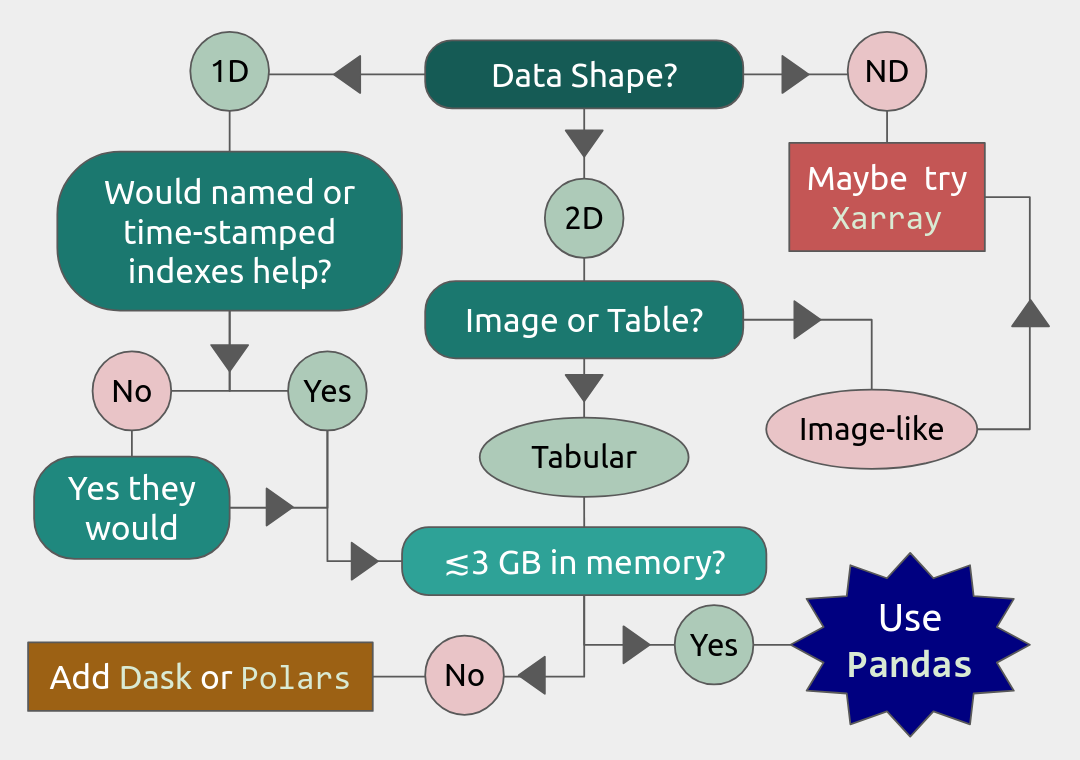
To know if Pandas is the right tool for your job, you can consult the flowchart below.

We will also have a short session after this on plotting with Seaborn, a package for easily making publication-ready statistical plots with Pandas data structures.

Introductory Topics (Review)

Important Data Types and Object Classes

The main object classes of Pandas are Series and DataFrame. There is also a separate object class called Index for the row indexes/labels and column labels, if applicable. Data that you load from file will mainly be loaded into either Series or DataFrames. Indexes are typically extracted later if needed.

• pandas.Series(data, index=None, name=None, ...) instantiates a 1D array with customizable indexes (labels) attached to every entry for easy access, and optionally a name for later addition to a DataFrame as a column.

  • Indexes can be numbers (integer or float), strings, datetime objects, or even tuples. The default is 0-based integer indexing. Indexes are also a Pandas data type (the data type of the row and column labels)

• pandas.DataFrame(data, columns=None, index=None, ...) instantiates a 2D array where every column is a Series. All entries are accessible by column and row labels/indexes.

  • Any function that works with a DataFrame will work with a Series unless the function specifically requires column arguments.

  • Column labels and row indexes/labels can be safely (re)assigned as needed.

For the rest of this lesson, example DataFrames will be abbreviated as df in code snippets (and example Series, if they appear, will be abbreviated as ser).

Pandas assigns the data in a Series and each column of a DataFrame a datatype based on built-in or NumPy datatypes or other formatting cues. Important Pandas datatypes include the following.

• Numerical data are stored as float64 or int64. You can convert to 32-, 16-, and even 8-bit versions of either to save memory.

• The object datatype stores any of the built-in types str, Bool, list, tuple, and mixed data types. Malformed data are also often designated as object type.

  • A common indication that you need to clean your data is finding a column that you expected to be numeric assigned a datatype of object.

• Pandas has many functions devoted to time series, so there are several datatypes—datetime, timedelta, and period. The first two are based on NumPy data types of the same name , and period is a time-interval type specified by a starting datetime and a recurrence rate. Unfortunately, we won’t have time to cover these at depth.

There are also specialized datatypes for, e.g. saving on memory or performing windowed operations, including

• Categorical is a set-like datatype for non-numeric data with few unique values. The unique values are stored in the attribute .categories, that are mapped to a number of low-bit-size integers, and those integers replace the actual values in the DataFrame as it is stored in memory, which can save a lot on memory usage.

• Interval is a datatype for tuples of bin edges, all of which must be open or closed on the same sides, usually output by Pandas discretizing functions.

• Sparse[float64, <omitted>] is a datatype based on the SciPy sparse matrices, where <omitted> can be NaN, 0, or any other missing value placeholder. This placeholder value is stored in the datatype, and the DataFrame itself is compressed in memory by not storing anything at the coordinates of the missing values.

This is far from an exhaustive list.

Loading/Creating DataFrames

Most of the time, Series and DataFrames will be loaded from files, not made from scratch. To review, the following table lists I/O functions for a few of the most common data formats; the full table with links to the documentation pages for each function can be found here. Input and output functions are sometimes called readers and writers, respectively. The read_csv() is by far the most commonly used since it can read any text file with a specified delimiter (comma, tab, or otherwise).

Typ1e	Data Description	Reader	Writer
text	CSV / ASCII text with standard delimiter	read_csv(path_or_url, sep=',', **kwargs)	to_csv(path, **kwargs)
text	JSON	read_json()	to_json(path, **kwargs)
SQL	SQLite table or query	read_sql()	to_sql(path, **kwargs)
binary	MS Excel/OpenDocument	read_excel(path_or_url, sheet_name=0, **kwargs)	to_excel(path, **kwargs)
binary	HDF5 Format	read_hdf()	to_hdf(path, **kwargs)
binary	Apache Parquet	read_parquet()	to_parquet()

Most of these functions have several dozen possible kwargs. It is left to the reader to determine which kwargs are needed. Most kwargs in a given reader function also appear in the corresponding writer function, and serve the same purpose.

Tip

Most of the text readers above, and the Excel reader, have kwargs that let you choose to load only some of the data, namely nrows and usecols.

• nrows lets you read in only the first n rows with their column headers, where $n ge 0$. If $n=0$, only the column names will be returned. This is a very efficient way to inspect large datasets.

• usecols is the same as in NumPy’s loadtxt() and genfromtxt() functions, i.e., it selects columns by position index and returns a data structure containing only those columns of data.

Tip

Most of the above reader/writer functions were chosen not only because they are commonly used, but because, apart from read_excel(), these support chunking for data sets that are larger than memory. Chunking is the act of performing operations, including I/O, on fixed-row-count subsets of the data, assuming each row is independent. For more information see the documentation on using chunking

In most reader functions, including index_col=0 sets the first column as the row labels, and the first row is assumed to contain the list of column names by default. If you forget to set one of the columns as the list of row indexes during import, you can do it later with df.set_index('column_name').

Exercise

Code along! Open your preferred IDE and load the provided file exoplanets_5250_EarthUnits_fixed.csv into DataFrame df. Then, save df to a text (.txt) file with a tab (\t) separator.

import pandas as pd
df = pd.read_csv('exoplanets_5250_EarthUnits_fixed.csv',index_col=0)
df.to_csv('./docs/day3/exoplanets_5250_EarthUnits.txt', sep='\t',index=True)

Creating DataFrames in Python. Building a DataFrame or Series from scratch is also easy. Lists and arrays can be converted directly to Series and DataFrames, respectively.

• Both pd.Series() and pd.DataFrame() have an index kwarg to assign a list of numbers, names, times, or other hashable keys to each row.

• You can use the columns kwarg in pd.DataFrame() to assign a list of names to the columns of the table. The equivalent for pd.Series() is just name, which only takes a single value and doesn’t do anything unless you plan to join that Series to a larger DataFrame.

• Dictionaries and record arrays can be converted to DataFrames with pd.DataFrame.from_dict(myDict) and pd.DataFrame.from_records(myRecArray), respectively, and the keys will automatically be converted to column labels.

Exercise

Code along! In your preferred IDE, recreate the DataFrame shown below and view it with a print statement.

import numpy as np
import pandas as pd
df = pd.DataFrame( np.arange(1,13).reshape((4,3)), index=['w','x','y','z'], columns=['a','b','c'] )
print(df)

    a   b   c
w   1   2   3
x   4   5   6
y   7   8   9
z  10  11  12

It is also possible (and occasionally necessary) to convert DataFrames and Series to NumPy arrays, dictionaries, record arrays, or strings with the methods .to_numpy(), .to_dict(), to_records(), and to_string(), respectively.

Inspection and Memory Usage

The main data inspection functions for DataFrames (and Series) are as follows:

• df.head() (or df.tail()) prints first (or last) 5 rows of data with row and column labels, or accepts an integer argument to print a different number of rows.

• df.info() prints the number of rows with their first and last index values; titles, index numbers, valid data counts, and datatypes of columns; and the estimated size of df in memory. Note: do not rely on this memory estimate if your dataframe contains non-numeric data (see below).

• df.describe() prints summary statistics for all the numerical columns in df.

• df.nunique() prints counts of the unique values in each column.

• df.value_counts() prints each unique value and the number of of occurrences for every combination of row and column values for as many of each as are selected (usually applied to just a couple of columns at a time at most)

• df.memory_usage() returns the estimated memory usage per column (see important notes below).

Important

The memory_usage() Function

df.memory_usage(deep=False) returns the estimated memory usage of each column, but with the default deep=False, this includes the sizes of pointers to non-numeric data, but not the full sizes of strings and other non-numeric data. The sum of these per-column estimates is the same as what is reported by df.info(), which is an significant underestimate. This is because numeric columns are fixed width in memory and can be stored contiguously, but object-type columns are variable in size, so only pointers can be stored at the location of the main DataFrame in memory. The strings that those pointers refer to are kept elsewhere. With deep=True, the sizes of strings and other non-numeric data are factored in, giving a much better estimate of the total size of df in memory.

import numpy as np
import pandas as pd
df = pd.read_csv('./docs/day3/exoplanets_5250_EarthUnits.csv',index_col=0)
print(df.info())
print('\n',df.memory_usage())
print('\n Compare: \n',df.memory_usage(deep=True))

<class 'pandas.core.frame.DataFrame'>
Index: 5250 entries, 11 Comae Berenices b to YZ Ceti d
Data columns (total 10 columns):
 #   Column             Non-Null Count  Dtype  
---  ------             --------------  -----  
 0   distance           5233 non-null   float64
 1   star_mag           5089 non-null   float64
 2   planet_type        5250 non-null   object 
 3   discovery_yr       5250 non-null   int64  
 4   mass_ME            5250 non-null   object 
 5   radius_RE          5250 non-null   object 
 6   orbital_radius_AU  4961 non-null   float64
 7   orbital_period_yr  5250 non-null   float64
 8   eccentricity       5250 non-null   float64
 9   detection_method   5250 non-null   object 
dtypes: float64(5), int64(1), object(4)
memory usage: 451.2+ KB
None

 Index                42000
distance             42000
star_mag             42000
planet_type          42000
discovery_yr         42000
mass_ME              42000
radius_RE            42000
orbital_radius_AU    42000
orbital_period_yr    42000
eccentricity         42000
detection_method     42000
dtype: int64

 Compare: 
 Index                317502
distance              42000
star_mag              42000
planet_type          313545
discovery_yr          42000
mass_ME              282482
radius_RE            284294
orbital_radius_AU     42000
orbital_period_yr     42000
eccentricity          42000
detection_method     306608
dtype: int64

Operations

Pandas DataFrames and Series have a vast library of function methods that are evaluated vector-wise (whole columns or rows at once) automatically. In lieu of in-depth discussion (provided by a separate course, “An Introduction to Pandas for Data Science”), important groups of operations and links to official documentation on their use are provided below. Users are encouraged to refer to these links in later exercises demonstrating how to make them run more efficiently on HPC systems. Iteration through loops is costly and usually avoidable.

String OperationsStatistical FunctionsBinary/Comparative MethodsUser-Defined Functions

Most built-in string methods can be applied column-wise to Pandas data structures (Series, Index, or columns of DataFrames) using .str.<method>(), where .str. is an accessor. Click here for complete documentation about working with text data in Pandas.

HPC-Specific Topics

Efficient Data Types

Categorical data. Categorical type maps all the unique values of a column to short numerical codes in the column’s place in memory, stores the codes in the smallest integer format that fits the largest-valued code, and only converts the codes to the associated strings when the data are printed. This data type is extremely efficient when the number of unique values are small relative to the size of the data set, but it is not recommended when half or more of the data values are unique.

• To convert a column in an existing Dataframe, simply set that column equal to itself with .astype('category') at the end. If defining a new Series that you want to be categorical, simply include dtype='category'.

• To get attributes or call methods of Categorical data, use the .cat accessor followed by the attribute or method. E.g., to get the category names as an index object, use df['cat_col'].cat.categories.

• .cat methods include operations to add, remove, rename, and even rearrange categories in a specific hierarchy.

• The order of categories can be asserted either in the definition of a Categorical object to be used as the indexes of a series, by calling .cat.as_ordered() on the Series if you’re happy with the current order, or by passing a rearranged or even a completely new list of categories to either .cat.set_categories([newcats], ordered=True) or .cat.reorder_categories([newcats], ordered=True).

  • When an order is asserted, it becomes possible to use .min() and .max() on the categories.

import pandas as pd
import numpy as np
df = pd.read_csv('./docs/day3/exoplanets_5250_EarthUnits_fixed.csv',index_col=0)
print("Before:\n", df['planet_type'].memory_usage(deep=True))
# Convert planet_type to categorical
ptypes=df['planet_type'].astype('category')
print("After:\n", ptypes.memory_usage(deep=True))
# assert order (coincidentally alphabetical order is also reverse mass-order)
ptypes = ptypes.cat.reorder_categories(ptypes.cat.categories[::-1], ordered=True)
print(ptypes)

Before:
 631047
After:
 323219
#name
11 Comae Berenices b      Gas Giant
11 Ursae Minoris b        Gas Giant
14 Andromedae b           Gas Giant
14 Herculis b             Gas Giant
16 Cygni B b              Gas Giant
                           ...     
XO-7 b                    Gas Giant
YSES 2 b                  Gas Giant
YZ Ceti b               Terrestrial
YZ Ceti c               Super Earth
YZ Ceti d               Super Earth
Name: planet_type, Length: 5250, dtype: category
Categories (5, object): ['Unknown' < 'Terrestrial' < 'Super Earth' < 'Neptune-like' < 'Gas Giant']

• Numerical data can be recast as categorical by binning it with pd.cut() or pd.qcut(), and these bins can be used to create GroupBy objects. Bins created like this are automatically assumed to be in ascending order.

Sparse Data. If you have a DataFrame where around half or more of the entries are NaN or a filler value, you can use the SparseArray format or SparseDtype to save memory. Initialize Series or DataFrames as SparseDtype by setting the kwarg dtype=pd.SparseDtype(dtype=np.float64, fill_value=None) in the pd.Series() or pd.DataFrame() initialization functions, or call the method .astype(pd.SparseDtype("float", fill_value)) on an existing Series or DataFrame. Data of SparseDtype have a .sparse accessor in much the same way as Categorical data have .cat. Most NumPy universal functions also work on Sparse Arrays. Other methods and attributes include:

• df.sparse.density: prints fraction of data that are non-NaN

• df.sparse.fill_value: prints fill value for NaNs, if any (if None, it returns NaN)

• df.sparse.from_spmatrix(data): makes a new SparseDtype DataFrame from a SciPy sparse matrix

• df.sparse.to_coo(): converts a DataFrame (or Series) to sparse SciPy COO type (more on those here)

This example shows the difference in memory usage between a 1000x1000 identity matrix as a regular NumPy array and as a SparseDtype DataFrame:

import pandas as pd
import numpy as np
import sys
a = np.diag( np.random.rand(1000) )
print("Regular memory usage as Numpy array: ", sys.getsizeof(a))
spdf = pd.DataFrame(a, dtype=pd.SparseDtype(dtype=np.float64, fill_value=0))
print("Memory usage as SparseDtype DataFrame: ", spdf.memory_usage(deep=True).sum())

Regular memory usage as Numpy array:  8000128
Memory usage as SparseDtype DataFrame:  12132

Automatic Multi-Threading with Numba

If Numba is installed, setting engine=numba in functions can boost performance if the function has to be run multiple times over several columns, particularly if you can set engine_kwargs={"parallel": True}. Types of functions that this works for include:

• Statistical functions like mean(), median(), and std(), which can be applied to the whole data set or to rolling windows.

• Complex functions, or user-defined functions decorated with @jit, applied via .agg(), .transform(), .map(), or .apply().

Parallel function evaluation occurs column-wise, so performance will be boosted if and only if the function is repeated many times over many columns. For small datasets, the added overhead can worsen performance.

Here is a (somewhat scientifically nonsensical) example using the exoplanets DataFrame to show the speed-up for 5 columns.

import numpy as np
import pandas as pd
df = pd.read_csv('./docs/day3/exoplanets_5250_EarthUnits_fixed.csv',index_col=0)
import numba
numba.set_num_threads(4)
stuff =  df.iloc[:,4:9].sample(n=250000, replace=True, ignore_index=True)
%timeit stuff.rolling(500).mean()
%timeit stuff.rolling(500).mean(engine='numba', engine_kwargs={"parallel": True})

24 ms ± 322 μs per loop (mean ± std. dev. of 7 runs, 10 loops each)

8.2 ms ± 335 μs per loop (mean ± std. dev. of 7 runs, 1 loop each)

Speed-up with Cython

The Cython package lets Python code be compiled into C with minimal additional code. The compiled code can then run markedly faster depending on the application and whether or not variables are declared with static data types. The Pandas documentation on Cython shows an example using Jupyter, <https://pandas.pydata.org/pandas-docs/stable/user_guide/enhancingperf.html#cython-writing-c-extensions-for-pandas> but the typical use case requires writing a .pyx file, compiling it with a setup.py script, and executing the compiled file from a Slurm script or the bash shell.

(TBC; see https://cython.readthedocs.io/en/stable/src/tutorial/cython_tutorial.html https://cython.readthedocs.io/en/stable/src/tutorial/array.html#array-array and https://cython.readthedocs.io/en/stable/src/tutorial/memory_allocation.html#memory-allocation )

Getting Dummy Variables for Machine Learning

ML programs like TensorFlow and PyTorch take Series/DataFrame inputs, but they generally require numeric input. If some of the variables that you want to predict are categorical (e.g. species, sex, or some other classification), they need to be converted to a numerical form that TensorFlow and PyTorch can use. Standard practice is turn a categorical variable with N unique values into N or N-1 boolean columns, where a row entry that was assigned a given category value has a 1 or True in the boolean column corresponding to that category and 0 or False in all the other boolean category columns.

The Pandas function that does this is pd.get_dummies(data, dtype=bool, drop_first=False, prefix=pref, columns=columns).

• dtype can be bool (default, less memory), float (more memory usage), int (same memory as float), or a more specific string identifier like 'float32' or 'uint16'

• drop_first, when True, lets you get rid of one of the categories on the assumption that not fitting any of the remaining categories is perfectly correlated with fitting the dropped category. Be aware that the only way to choose which column is dropped is to rearrange the original data so that the column you want dropped is first.

• prefix is just a set of strings you can add to dummy column names to make clear which ones are related.

• If nothing is passed to columns, Pandas will try to convert the entire DataFrame to dummy variables, which is usually a bad idea. Always pass the subset of columns you want to convert to columns.

Let’s say you did an experiment where you tested 100 people to see if their preference for Coke or Pepsi correlated with whether the container it came in was made of aluminum, plastic, or glass, and whether it was served with or without ice.

from random import choices
import pandas as pd
sodas = choices(['Coke','Pepsi'],k=100)
containers = choices(['aluminum','glass','plastic'],k=100)
ices = choices([1, 0],k=100) ###already boolean
soda_df = pd.DataFrame(list(zip(sodas,containers,ices)),
                       columns=['brand','container_material','with_ice'])
print(soda_df.head())
print("\n Memory usage:\n",soda_df.memory_usage(deep=True),"\n")
dummy_df = pd.get_dummies(soda_df, drop_first=True, columns=['brand','container_material'],
                          prefix=['was','in'], dtype=int)
print("Dummy version:\n",dummy_df.head())
print("\n Memory usage:\n",dummy_df.memory_usage(deep=True))

   brand container_material  with_ice
0  Pepsi            plastic         0
1  Pepsi              glass         0
2  Pepsi              glass         0
3  Pepsi           aluminum         0
4   Coke            plastic         1

 Memory usage:
 Index                  132
brand                 5344
container_material    5592
with_ice               800
dtype: int64 

Dummy version:
    with_ice  was_Pepsi  in_glass  in_plastic
0         0          1         0           1
1         0          1         1           0
2         0          1         1           0
3         0          1         0           0
4         1          0         0           1

 Memory usage:
 Index         132
with_ice      800
was_Pepsi     800
in_glass      800
in_plastic    800
dtype: int64

Dummy variables can also be converted back to categorical variable columns with pd.from_dummies() as long as their column names had prefixes to group related variables. But given the memory savings, you might not want to.