Big data with Python
“Learning outcomes”
Learners
can allocate resources sufficient to data size
can decide on useful file formats
can use data-chunking as technique
know where to learn more
“For teacher”
Preliminary timings. Starting at 13.00
Intro 10 min
Memory 5
Exercise Allocation 10
Files 5
Exercise files 10
Packages 5
Dask 5
BREAK 15min 13.50-14.05
Exercise Dask 30
Introduction
High-Performance Data Analytics (HPDA)
What is it?
High-performance data analytics (HPDA), a subset of high-performance computing which focuses on working with large data.
The data can come from either computer models and simulations or from experiments and observations, and the goal is to preprocess, analyse and visualise it to generate scientific results.
“Big data refers to data sets that are too large or complex to be dealt with by traditional data-processing application software. […]
Big data analysis challenges include capturing data, data storage, data analysis, search, sharing, transfer, visualization, querying, updating, information privacy, and data source.” (from Wikipedia)
Discussion
Do you already work with large data sets?
Why we need to take special actions
Discussion
What can limit us?
What the constraints are
storage
memory
What do we need to cover??
storage –> make more effective files
- reading into memory
–> read just parts of files into memory
–> chunking
allocate more memory
Solutions and tools
- Allocate enough RAM
If you are running ready tools
or cannot update code or use other packages
Choose file format for reading and writing
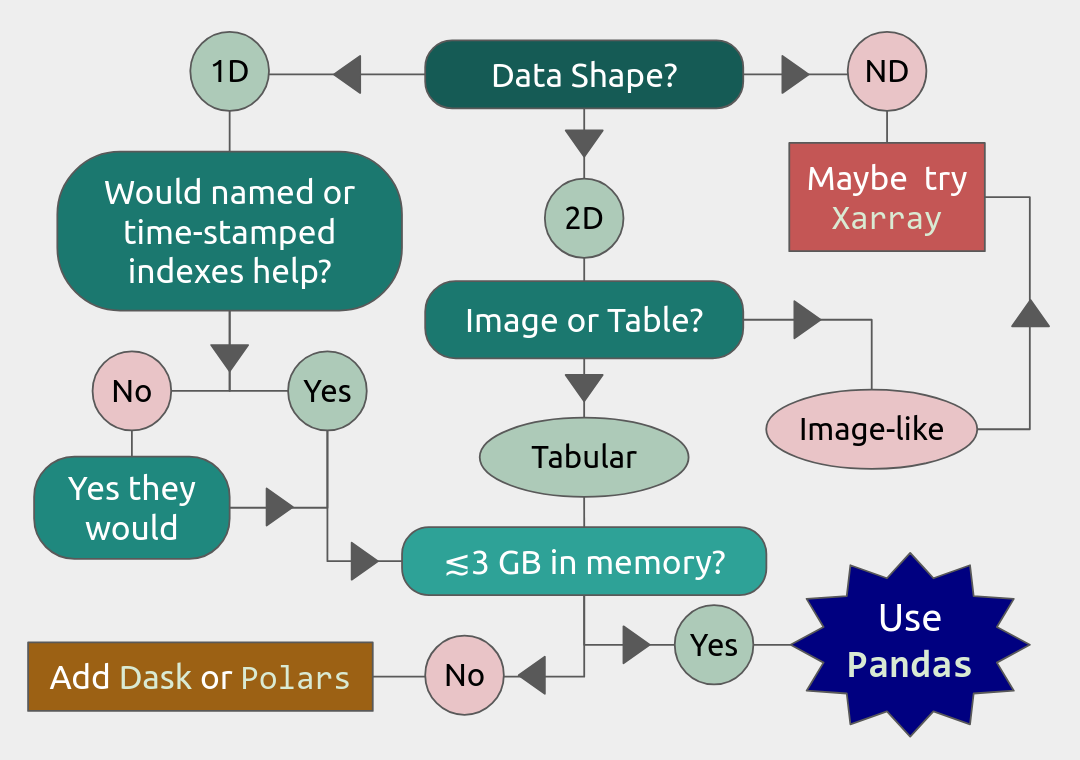
Choose the right Python package
Is chunking suitable?
Allocating RAM
How much is actually loaded into the working memory (RAM)
Is more data in variables created during the run or work?
Discussion
Have you seen the Out-of-memory (OOM) error?
What to do
By allocating many cores on a node will give you more available memory
If the order 128 GB is not enough there are so-called fat nodes with at least 512 GB and up to 3 TB.
- On some clusters you do not have to request additional CPUs to get additional memory. Use the
slurmoptions --memor--mem-per-cpu
- On some clusters you do not have to request additional CPUs to get additional memory. Use the
Important
You do not have to explicitly run threads or other parallelism (see
Allocating several nodes for one one big memory problem is not useful. (Unless you are “chunking”)
Note that shared memory among the cores works within node only.
Principles
Use the Slurm options for either “BATCH”, “INTERACTIVE” from command line or from OnDemand GUIs.
- Allocate RAM using the full node RAM divided by number of course principle
Ex: 128 GB with 20 cores –> 6.4 GB per core
Allocate number of cores to cover your needs.
-n <number>
- Request the memory needed and choose number of cores
--mem=<size>[K|M|G|T]Example:
--mem=150G
- Request the memory-per-core needed and choose number of cores
--mem-core=<size>[K|M|G]Example:
--mem-per-cpu=16G
- Request a “FAT” node.
Typically you can only allocate a full node here, no core parts.
You ask here for a non-default partition.
How to do this, search your cluster documentation, see exercise below.
Example for Tetralith with one core but 50 GB RAM for one hour
interactive -A naiss2026-4-66 --mem 50G -t 1:0:0
Note
“core-hours” drawn from your project may be set to the maximum of “number of cores” and “memory part of node” requested.
So there is no win to ask for one core but much memory!
Exercise: Memory allocation (10 min)
1a. Log in to a Desktop (ThinLinc or OnDemand) (see Log in and other preparations)
Links and addresses
Tetralith (ThinLinc client:
tetralith.nsc.liu.se)Dardel (ThinLinc client:
dardel-vnc.pdc.kth.se)Alvis (https://alvis.c3se.chalmers.se/)
Bianca (https://bianca.uppmax.uu.se/)
Pelle (https://pelle-gui.uppmax.uu.se/)
Cosmos (ThinLinc client:
cosmos-dt.lunarc.lu.se)Kebnekaise (https://portal.hpc2n.umu.se/public/landing_page.html)
1b. If You cannot use a desktop it is all fine with a command line: ssh ...
Discussion
Take some time to find out the answers for your specific cluster for the questions below, using the table of hardware below.
Table of hardware
Hardware
Technology |
Kebnekaise |
Pelle |
Bianca |
Cosmos |
Tetralith |
Dardel |
Alvis |
|---|---|---|---|---|---|---|---|
Cores/compute node |
28 (72 for largemem, 128/256 for AMD Zen3/Zen4) |
48 (96 with hyperthreading/SMT) |
16 |
48 |
32 |
128 |
many different (updated soon) |
Memory/compute node |
128-3072 GB |
768-3072 GB |
128-512 GB |
256-512 GB |
96-384 GB |
256-1760 GB |
many different |
GPU |
NVidia V100, A100, A6000, L40s, H100, A40, AMD MI100 |
NVidia L40s, H100, T4, A2) |
NVidia A100 |
NVidia A100 |
NVidia T4 |
4 AMD Instinct™ MI250X á 2 GCDs |
many different |
How much memory do I get per core?
Divide GB RAM of the booked node with number of cores.
- Example: 128 GB node with 16 cores
~8 GB per core
- NOTE: You may get less due to background system threads running in the background.
Example: On Bianca you may get 7 GB instead of 8 GB.
How much memory do I get with 5 cores?
Multiply the RAM per core with number of allocated cores..
- Example: ~8 GB per core
~40 GB
Do you remember how to allocate several cores?
Slurm option
-n <number of cores>
Actually start an interactive session with 4 cores for 3 hours.
We will use it for the exercises later.
Since it may take some time to get the allocation we do it now already!
Follow the best procedure for your cluster, e.g. from command-line or OnDemand.
Continue with the other exercises below, while session is waiting to be started.
How?
Start with the command
sallocorinteractive(depending on system) followed by the Slurm options:-t 3:0:0-n 4-A <proj>-p <partition>may be needed in some clustersDardel:
-p shared
Compute project numbers in this workshop
How to get a node with more RAM?
See local HPC center documentation in how to do so!
Try first to search or navigate the pages
Documentation links
Commands
-C fat --exclusive (384 GiB)
-p memory --mem=440GB-p memory --mem=880GB-p memory --mem=1760GB
-C MEM512-C MEM1536
-C mem256GB-C mem512GB
-p fat -C 2TB-p fat -C 3TB
Part of GPU partitions
INTEL CPUs+A100 GPUs (384 GB):
-p gpua100AMD CPUs+A100 GPUs (512 GB):
-p gpua100
-C largemem
Note
We recommend a desktop environment for speed of the graphics.
connecting from local terminal with “ssh -X” (X11 forwarding) can be be used but is slower.
File formats
Bits and Bytes
The smallest building block of storage and memory (RAM) in the computer is a bit, which stores either a 0 or 1.
Normally a number of 8 bits are combined in a group to make a byte.
One byte (8 bits) can represent/hold at most 2^8 distinct values. Organising bytes in different ways can represent different types of information, i.e. data.
Numerical data
Different numerical data types (e.g. integer and floating-point numbers) can be represented by bytes. The more bytes we use for each value, the larger is the range or precision we get, but more bytes require more memory.
- DataTypes
16-bit: short (integer)
32-bit: Int (integer)
32-bit: Single (floating point)
64-bit: Double (floating point)
For some use cases, the precision is not that important, 1% error, or so, is not that crucial. Faster and less data storage!
Text data
- DataTypes
8-bit: char
more
When it comes to text data, the simplest character encoding is ASCII (American Standard Code for Information Interchange) and was the most common character encodings until 2008 when UTF-8 took over.
The original ASCII uses only 7 bits for representing each character and therefore encodes only 128 specified characters. Later it became common to use an 8-bit byte to store each character in memory, providing an extended ASCII.
As computers became more powerful and the need for including more characters from other languages like Chinese, Greek and Arabic became more pressing, UTF-8 became the most common encoding. UTF-8 uses a minimum of one byte and up to four bytes per character.
Data and storage format
In real scientific applications, data is complex and structured and usually contains both numerical and text data. Here we list a few of the data and file storage formats commonly used.
Tabular data
A very common type of data is “tabular data”.
Tabular data is structured into rows and columns.
Each column usually has a name and a specific data type while each row is a distinct sample which provides data according to each column (including missing values).
The simplest and most common way to save tabular data is via the so-called CSV (comma-separated values) file.
Gridded data
Gridded data is another very common data type in which numerical data is normally saved in a multi-dimensional rectangular grid. Most probably it is saved in one of the following formats:
more
Hierarchical Data Format (HDF5) - Container for many arrays
Network Common Data Form (NetCDF) - Container for many arrays which conform to the NetCDF data model
Zarr - New cloud-optimized format for array storage
Meta data
Metadata consists of various information about the data. Different types of data may have different metadata conventions.
more
In Earth and Environmental science, there are widespread robust practices around metadata. For NetCDF files, metadata can be embedded directly into the data files. The most common metadata convention is Climate and Forecast (CF) Conventions, commonly used with NetCDF data.
When it comes to data storage, there are many types of storage formats used in scientific computing and data analysis. There isn’t one data storage format that works in all cases, so choose a file format that best suits your data.
CSV (comma-separated values)
Best use cases: Sharing data. Small data. Data that needs to be human-readable.
Key features
Type: Text format Packages needed: NumPy, Pandas Space efficiency: Bad Good for sharing/archival: Yes
more
- Tidy data:
Speed: Bad Ease of use: Great
- Array data:
Speed: Bad Ease of use: OK for one or two dimensional data. Bad for anything higher.
HDF5 (Hierarchical Data Format version 5)
HDF5 is a high performance storage format for storing large amounts of data in multiple datasets in a single file.
It is especially popular in fields where you need to store big multidimensional arrays such as physical sciences.
Best use cases: Working with big datasets in array data format.
Key features
Type: Binary format
Packages needed: Pandas, PyTables, h5py
Space efficiency: Good for numeric data.
Good for sharing/archival: Yes, if datasets are named well.
more
- Tidy data:
Speed: Ok
Ease of use: Good
- Array data:
Speed: Great
Ease of use: Good
NETCDF4 (Network Common Data Form version 4)
NetCDF4 is a data format that uses HDF5 as its file format, but it has standardized structure of datasets and metadata related to these datasets.
This makes it possible to be read from various different programs.
Best use cases: Working with big datasets in array data format. Especially useful if the dataset contains spatial or temporal dimensions. Archiving or sharing those datasets.
Key features
Type: Binary format
Packages needed: Pandas, SciPy, netCDF4/h5netcdf, xarray
Space efficiency: Good for numeric data.
Good for sharing/archival: Yes.
more
- Tidy data:
Speed: Ok
Ease of use: Good
- Array data:
Speed: Good
Ease of use: Great
NetCDF4 is by far the most common format for storing large data from big simulations in physical sciences.
The advantage of NetCDF4 compared to HDF5 is that one can easily add additional metadata, e.g. spatial dimensions (x, y, z) or timestamps (t) that tell where the grid-points are situated. As the format is standardized, many programs can use this metadata for visualization and further analysis.
See also
ENCCS course “HPDA-Python”: Scientific data
Aalto Scientific Computing course “Python for Scientific Computing”: Xarray
Exercise file formats (10 minutes)
Reading NetCDF files
Read: https://stackoverflow.com/questions/49854065/python-netcdf4-library-ram-usage
What about using NETCDF files and memory?
View file formats
Go over file formats and see if some are more relevant for your work.
Overview of common data formats
Name:
|
Human
readable:
|
Space
efficiency:
|
Arbitrary
data:
|
Tidy
data:
|
Array
data:
|
Long term
storage/sharing:
|
|---|---|---|---|---|---|---|
Pickle |
❌ |
🟨 |
✅ |
🟨 |
🟨 |
❌ |
CSV |
✅ |
❌ |
❌ |
✅ |
🟨 |
✅ |
Feather |
❌ |
✅ |
❌ |
✅ |
❌ |
❌ |
Parquet |
❌ |
✅ |
🟨 |
✅ |
🟨 |
✅ |
npy |
❌ |
🟨 |
❌ |
❌ |
✅ |
❌ |
HDF5 |
❌ |
✅ |
❌ |
❌ |
✅ |
✅ |
NetCDF4 |
❌ |
✅ |
❌ |
❌ |
✅ |
✅ |
JSON |
✅ |
❌ |
🟨 |
❌ |
❌ |
✅ |
Excel |
✅ |
❌ |
❌ |
🟨 |
❌ |
🟨 |
🟨 |
🟨 |
❌ |
❌ |
❌ |
✅ |
Legend
✅ : Good
🟨 : Ok / depends on a case
❌ : Bad
Adapted from Aalto university’s Python for scientific computing
Would you look at or change to other file formats than you use today and why?
(optional)
Start Jupyter or just a Python shell and
Go though and test the lines at the page at https://docs.scipy.org/doc/scipy-1.13.1/reference/generated/scipy.io.netcdf_file.html
Computing efficiency with Python
Python is an interpreted language, and many features (dynamical typing, flexible data structures) that make development rapid with Python are a result of that, with the price of reduced performance in many cases.
There are some packages that are more efficient than Numpy and Pandas.
SciPy is a library that builds on top of NumPy.
It contains a lot of interfaces to battle-tested numerical routines written in Fortran or C, as well as Python implementations of many common algorithms.
Reads NETCDF!
Xarray package
xarray is a Python package that builds on NumPy but adds labels to multi-dimensional arrays.
labels in the form of dimensions, coordinates and attributes on top of raw NumPy-like multidimensional arrays, which allows for a more intuitive, more concise, and less error-prone developer experience.
borrows from the Pandas package for labelled tabular data and integrates tightly with
daskfor parallel computing.particularly tailored to working with NetCDF files.
work for another file formats as well
Explore it a bit in the (optional) exercise below!
Dask
How to use more resources than available?
Remember this image? ;-)
Dask is very popular for data analysis and is used by a number of high-level Python libraries.
2 parts:
- Dask Clusters
Dynamic task scheduling optimized for computation. Similar to other workflow management systems, but optimized for interactive computational workloads.
- “Big Data” Collections
Like parallel arrays, dataframes, and lists that extend common interfaces like NumPy, Pandas, or Python iterators to larger-than-memory or distributed environments. These parallel collections run on top of dynamic task schedulers.
Dask Collections
Dask provides dynamic parallel task scheduling and three main high-level collections:
dask.array: Parallel NumPy arraysscales NumPy (see also xarray)
dask.dataframe: Parallel Pandas DataFramesscales Pandas workflows
dask.bag: Parallel Python List
See also
dask_ml package: Dask-ML provides scalable machine learning in Python using Dask alongside popular machine learning libraries like Scikit-Learn, XGBoost, and others.
Dask.distributed: Dask.distributed is a lightweight library for distributed computing in Python. It extends both the concurrent.futures and dask APIs to moderate sized clusters.
dask.arrays
A Dask array looks and feels a lot like a NumPy array.
- However, a Dask array uses the so-called “lazy” execution mode, which allows one to
build up complex, large calculations symbolically
before turning them over the scheduler for execution.
Chunks
Dask divides arrays into many small pieces (chunks), as small as necessary to fit it into memory.
Operations are delayed (lazy computing) e.g.
tasks are queued and no computation is performed until you actually ask values to be computed (for instance print mean values).
Then data is loaded into memory and computation proceeds in a streaming fashion, block-by-block.
And data is gathered in the end.
Tools like Dask and xarray handle “chunking” automatically.
Note that number of chunks does not need to be equal to number of cores.
Big file → split into chunks → parallel workers → results combined.
To think of
Chunk size and number of them affect the performance due to overhead/administration of the chunking and combination.
Briefly explain what happens when a Dask job runs on multiple cores.
Example from dask.org
# Arrays implement the Numpy API
import dask.array as da
x = da.random.random(size=(10000, 10000),
                     chunks=(1000, 1000))
x + x.T - x.mean(axis=0)
# It runs using multiple threads on one node.
# It could also be distributed to multiple nodes
Polars package
Polars is a Python package that presents itself as Blazingly Fast DataFrame Library
Utilizes all available cores on your machine.
Optimizes queries to reduce unneeded work/memory allocations.
Handles datasets much larger than your available RAM.
A consistent and predictable API.
Adheres to a strict schema (data-types should be known before running the query).
Exercises: Packages
Set up the environment
Important
Interactive use (Recommended)
Follow the instructions here: https://docs.hpc2n.umu.se/tutorials/connections/#example__-__jupyter__with__extra__modules.
Add these lines in the batch script
module load SciPy-bundle/2023.07 matplotlib/3.7.2 Tkinter/3.11.3
Continue and start Jupyter
And install
polars,dask&xarrayto~/.local/if you don’t already have it
! pip install --user xarray
! pip install --user dask
! pip install --user polars
You may have to restart the Jupyter kernel (or even Jupyter session) to be able to load the just installed package(s).
Important
Interactive Use (Recommended)
Start a Thinlinc session and open one of Spyder, Jupyter Lab, or VSCode from the On-Demand applications menu as discussed in the On-Demand lesson from Day 2. Spyder and Jupyter Lab are configured to load Xarray and Dask and all their dependencies automatically via the latest version of Anaconda, whereas VSCode requires modules to be selected to load as part of the additional job settings.
Continue and start Jupyter
And install
polarsto~/.local/if you don’t already have it
! pip install --user polars
You may have to restart the Jupyter kernel (or even Jupyter session) to be able to be able to load the just instaleld package(s).
Non-Interactive Use
ml GCC/12.3.0 OpenMPI/4.1.5 xarray/2023.9.0 dask/2023.9.2
if you prefer pip-installed Python packages, or you can load
ml Anaconda3/2024.06-1
Important
General Use
module load dask/2024.9.1-gfbf-2024a xarray/2024.11.0-gfbf-2024a JupyterLab/4.2.5-GCCcore-13.3.0 polars/1.29.0-gfbf-2024a
This command also loads SciPy-bundle/2024.05-gfbf-2024a (which includes Numpy and Pandas) and matplotlib/3.9.2-gfbf-2024a, but not any IDEs.
Continue and start Jupyter as discussed in the interactive usage lesson on Day 2.
Important
General Use
You should for this session load
module load buildtool-easybuild/4.8.0-hpce082752a2 GCC/13.2.0 Python/3.11.5 SciPy-bundle/2023.11
Continue and start Jupyter
And install
dask&xarray(and polars) to~/.local/if you don’t already have it
! pip install --user xarray
! pip install --user dask
! pip install --user polars
Interactive Use
In a Thinlinc session, open a terminal and start
interactive -A [project_name] -t HHH:MM:SS
as discussed in the interactive usage lesson on Day 2. Once transferred to a compute node, do
module load buildtool-easybuild/4.8.0-hpce082752a2 GCC/13.2.0 Python/3.11.5 SciPy-bundle/2023.11 JupyterLab/4.2.0
or swap JupyterLab for your preferred IDE following the IDEs lesson from Day 2.
Jupyter Lab is only available on Dardel via ThinLinc.
As there are only 30 ThinLinc licenses available at this time, we recommend that you work on the exercises with a local installation on a personal computer.
Do not trust that a ThinLinc session will be available or that On-Demand applications run therein will start in time for you to keep up (it is not unusual for wait times to be longer than the requested walltime).
The exercises were written to work on a regular laptop. If you must work on Dardel, follow the steps below. The exercise prompts and their solutions are included on this page.
Important
General Use
For this session, you could load
ml cray-python/3.11.7 PDCOLD/23.12 matplotlib/3.8.2-cpeGNU-23.12
On Dardel, all cray-python versions include NumPy, SciPy, Pandas, and Dask, and do not have any prerequisites, but Seaborn is part of matplotlib/3.8.2-cpeGNU-23.12, which has PDCOLD/23.12 as a prerequisite. The versions available for cray-python and Matplotlib are limited because Dardel users are typically expected to build their own environments, but for this course, the installed versions are fine.
Interactive use with Thinlinc (If Available) :collapsible:
Start Jupyter from the menu and it will work
Default Anaconda3 has all packages needed for this lesson
Or use Spyder:
First start interactive session
salloc --ntasks=4 -t 0:30:00 -p shared --qos=normal -A naiss2025-22-934
salloc: Pending job allocation 9102757
salloc: job 9102757 queued and waiting for resources
salloc: job 9102757 has been allocated resources
salloc: Granted job allocation 9102757
salloc: Waiting for resource configuration
salloc: Nodes nid001057 are ready for job
Then ssh to the specific node, like
ssh nid001057Use the conda env you created in Exercise 2 in Use isolated environments
ml PDC/24.11
ml miniconda3/25.3.1-1-cpeGNU-24.11
export CONDA_ENVS_PATH="/cfs/klemming/projects/supr/courses-fall-2025/$USER/"
export CONDA_PKG_DIRS="/cfs/klemming/projects/supr/courses-fall-2025/$USER/"
source activate spyder-env
# If needed, install the packages here by: "conda install matplotlib pandas seaborn"
spyder &
Important
For this session, you should use the Alvis portal: https://alvis.c3se.chalmers.se/public/root/
Log in
Ask for Desktop (Compute) in left-hand side menu. Do not choose “Jupyter”, since it gives you a TensorFlow environment with Python 3.8.
Open a Terminal and load the following software modules
ml xarray/2024.11.0-gfbf-2024a dask/2024.9.1-gfbf-2024a
ml Jupyter-bundle/20250530-GCCcore-13.3.0
This will load matplotlib & SciPy-bundle on the fly!
Make a virtual environment
virtualenv polarsvenv --system-site-packages
. polarsvenv/bin/activate
pip install polars
python -m ipykernel install --user --name=polarsvenv --display-name="Test"
Then start jupyter-lab and a web browser will automatically open
jupyter-lab
Chunk sizes in Dask
The following example calculate the mean value of a random generated array.
Run the 2 examples and see the performance improvement by using dask.
import numpy as np
%%time
x = np.random.random((20000, 20000))
y = x.mean(axis=0)
import dask
import dask.array as da
%%time
x = da.random.random((20000, 20000), chunks=(1000, 1000))
y = x.mean(axis=0)
y.compute()
But what happens if we use different chunk sizes? Try out with different chunk sizes:
What happens if the dask chunks=``(20000,20000)``
What happens if the dask chunks=``(250,250)``
Choice of chunk size
The choice is problem dependent, but here are a few things to consider:
Each chunk of data should be small enough so that it fits comforably in each worker’s available memory. Chunk sizes between 10MB-1GB are common, depending on the availability of RAM. Dask will likely manipulate as many chunks in parallel on one machine as you have cores on that machine. So if you have a machine with 10 cores and you choose chunks in the 1GB range, Dask is likely to use at least 10 GB of memory. Additionally, there should be enough chunks available so that each worker always has something to work on.
On the otherhand, you also want to avoid chunk sizes that are too small as we see in the exercise. Every task comes with some overhead which is somewhere between 200us and 1ms. Very large graphs with millions of tasks will lead to overhead being in the range from minutes to hours which is not recommended.
(Optional) Xarray
Read when-to-use-xarray-over-numpy-for-medium-rank-multidimensional-data
Browse: https://docs.xarray.dev/en/v2024.11.0/getting-started-guide/why-xarray.html or change to more applicable version in drop-down menu to lower right.
Find something interesting for you! Test some lines if you want to!
Tips:
(Optional) Polars
- Browse https://docs.pola.rs/.
find something interesting for you! Test some lines if you want to!
Key features
Fast: Written from scratch in Rust
I/O: First class support for all common data storage layers
Intuitive API: Write your queries the way they were intended. Internally, there is a query optimizer.
Out of Core: streaming without requiring all your data to be in memory at the same time. I.e. chunking
Parallel: dividing the workload among the available CPU cores without any additional configuration.
GPU Support: Optionally run queries on NVIDIA GPUs
Apache Arrow support
Check if your cluster has Polars!
Solution
Check with
ml spider polarsIf it is installed it will show up as
--------------------------------------------------------------------
  polars:
--------------------------------------------------------------------
    Description:
      Polars is a blazingly fast DataFrame library for manipulating
      structured data. The core is written in Rust and this module
      provides its interface for Python.

     Versions:
        polars/1.28.1-gfbf-2024a
        polars/1.29.0-gfbf-2024a

--------------------------------------------------------------------
  For detailed information about a specific "polars" package (including
how to load the modules) use the module's full name.
  Note that names that have a trailing (E) are extensions provided by ot
her modules.
  For example:

     $ module spider polars/1.29.0-gfbf-2024a
--------------------------------------------------------------------
Load the module or install it in your present
condaorvenvenvironmentTry the most interesting examples here
Summary
Follow-up discussion
New learnings?
Useful file formats
Resources sufficient to data size
Data-chunking as technique if not enough RAM
Is Xarray/Polars/Dask useful for you?
Keypoints
- Allocate more RAM by asking for
Several cores or request
--memNodes with more RAM
Check job memory usage with
sacctorsstat. Check you documentation!
- File formats
No format fits all requirements
HDF5 and NetCDF good for Big data since it allows loading parts of the file into memory
Store temporary data in local scratch
($SNIC_TMP).- Packages
- xarray
can deal with 3D-data and higher dimensions
- Dask
uses lazy execution
Only use for processing very large amount of data
Chunking: Data source → Format choice → Load/Chunk → Process → Write
See also
ENCCS